Calculus II in practice: case studies and a project

This course has extended calculus in three directions: techniques for evaluating integrals (Lessons 1 and 2), applications of integration to geometry, mechanics, fluids and heat (Lessons 3, 4, 6 and 11), differential equations (Lesson 5), curves described parametrically and in polar form (Lesson 7), and infinite series, from Taylor series to complex exponentials and Fourier series (Lessons 8 to 10). Real problems rarely announce which of these tools they need. This final lesson works through three case studies, each combining several lessons, and then sets a course project in which you model an engineering system of your choice with the tools of the course. The modeling cycle described at the end of Calculus I (MATH-100, Lesson 12) applies throughout: state the question and assumptions, formulate the equations, solve, check against limiting cases and data, and communicate the result.

Case study 1: draining a spherical tank

Spherical tanks store liquefied gases, water and chemicals because a sphere holds the most volume for a given surface area and resists pressure efficiently. Suppose a spherical water tank of radius \(R = 1.5\) m, initially full, must be drained for inspection through a 50 mm sharp-edged outlet at the bottom with discharge coefficient 0.61. How long will it take?

• Geometry (Lesson 3): at depth \(h\) above the bottom, the horizontal cross-section is a circle of radius \(\sqrt{2Rh - h^2}\), so its area is \(A(h) = \pi(2Rh - h^2)\).
• Flow (Lesson 5): Torricelli's law gives the outflow \(C_d a\sqrt{2gh}\), and conservation of volume gives the separable equation \(A(h)\,\dfrac{dh}{dt} = -C_d a\sqrt{2gh}\).
• Integration: separating and integrating from full (\(h = 2R\)) to empty (\(h = 0\)) gives the drain time.

Case study 2: the ripple of a rectified supply

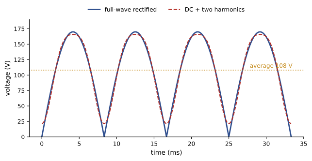
An AC-to-DC power supply first rectifies the mains voltage. A full-wave rectifier produces \(|V_p\sin\omega t|\), which has a large DC component but also large ripple. To design the filter that smooths it, the engineer needs to know how much of each frequency is present, a Fourier series problem (Lesson 10).

Case study 3: the length of a suspension cable

The main cables of a suspension bridge, which carry a nearly uniform load per horizontal meter, hang in a parabola. Engineers need the cable length to order the cable and to compute how much it stretches under load. For a span \(L\) with sag \(s\) at midspan, the cable is \(y = 4sx^2/L^2\) for \(-L/2 \le x \le L/2\), and its length is the arc length integral (Lesson 3):

This integral can be done exactly with a trigonometric or hyperbolic substitution (Lesson 2), but the result is cumbersome. Engineers instead expand the square root with the binomial series (Lesson 9), \(\sqrt{1 + u} \approx 1 + \tfrac{u}{2} - \tfrac{u^2}{8}\), and integrate term by term:

Common threads

The case studies share several lessons for practice. Each combined two or three topics from the course, so the ability to recognize which tools a problem needs matters as much as skill with any single technique. Each involved an approximation or an assumption (Torricelli flow, ideal rectification, a parabolic cable) that should be stated and checked. Each result was checked against a simpler estimate: the initial outflow rate, the size of the harmonics, the exact numerical length. And each answer was interpreted in terms of what an engineer would do with it: plan a drain-down, design a filter, order a cable.

The course project

Choose one of the following problems, or propose your own of similar scope with your instructor's approval, and write a technical report of about eight pages including figures.

• Project A: A storage tank. Choose a tank shape (horizontal cylinder, sphere, cone or cylinder with hemispherical ends). Derive its volume as a function of liquid depth (Lessons 2 and 3) and produce a gauge chart. Find the centroid of the liquid at several depths (Lesson 4) and the time to drain through a specified outlet (Lesson 5). Compare a Simpson's rule estimate of one integral with its exact value.
• Project B: A periodic signal. Choose a periodic waveform from engineering practice (a PWM output, a rectifier current, a cam lift profile, a daily temperature cycle). Compute its Fourier coefficients (Lesson 10), plot partial sums, find its RMS value and harmonic distortion using Parseval's theorem, and design a simple filter or analyze the response of a first-order system to it (Lessons 5 and 9).
• Project C: A structural or thermal element. Analyze a beam with a non-uniform load, or insulation on a pipe or tank, from first principles (Lesson 11): set up the governing integral or differential equation, solve it, check limiting cases, and investigate how the result depends on the main design parameters. Include a series approximation (Lesson 9) of a key result and assess its accuracy.
• Project D: A curve in design. Model a cam profile, a gear tooth, a road transition curve or a suspension cable with parametric or polar equations (Lesson 7); compute slopes, curvature-related quantities, arc length and enclosed area; and compare exact, series and numerical evaluations of any integral that has no elementary form.

Every report should state the problem and assumptions, derive the equations, present the calculations clearly with units, include at least two graphs, check results against limiting cases or independent estimates, analyze sensitivity to at least two parameters, and discuss limitations. Where you use software to evaluate integrals or sums, show that you have verified its results by hand calculation, differentiation or convergence checks.

Working with software

Each case study could be done in minutes with mathematical software, and engineers routinely use computer algebra, spreadsheets and numerical libraries for this kind of work. Software changes what an engineer must be good at, not whether calculus matters. Someone must set up the right integral or equation, choose sensible units and parameters, recognize when a result is implausible, and know which approximations are being made. In the spherical tank problem, for example, software would integrate whatever area function it was given; only an engineer who understands the geometry would notice an area formula that went negative above the equator. A practical workflow is to sketch the expected behavior first, compute with software, then check the output against a hand estimate, a limiting case or an independent method, and record the inputs so that others can reproduce the result. The course project asks for exactly this combination of analysis, computation and checking.

Looking ahead

The tools of this course carry directly into the second year of an engineering program. Multivariable calculus (MATH-209) extends integration to areas, volumes and surfaces in two and three dimensions, where the element method of Lessons 3, 4 and 11 becomes double and triple integrals. Differential equations (MATH-201) builds on Lesson 5 and on the complex exponentials of Lesson 9 to treat vibrations, circuits and control systems, and introduces the Laplace transform previewed in Lesson 6. Numerical methods (MATH-300) develops the numerical integration and series approximations used here into general algorithms. And the Fourier series of Lesson 10 lead to the Fourier transform in signals and systems. Calculus is not finished when this course ends: it becomes the language in which engineering is done.