
JS-201 · Lesson 1 of 12 · 26 min
Measuring algorithms and Big-O
▶ Video coming soon A video version of this lesson is on the way.
If the plan holds, the Riverside Community Food Hub will begin its second autumn with Brightwater Web Studio's software in daily use. The lunch counter page has taken orders since March 2027, Lucy Tran's office dashboard has shown the day's shifts since the April pilot, and in June the counter page, the dashboard client and the riverside-data library moved to TypeScript. Mira Castellanos, who joined Brightwater as an apprentice in September 2026, starts the second year of her apprenticeship in September 2027 with a new kind of work: making that code fast and correct as the Food Hub's data keeps growing.
Gareth Lindqvist, the senior developer and Mira's mentor, has planned a sixth block of Tuesday and Thursday sessions, from Tuesday, September 7 to Thursday, October 14, 2027. The subject is data structures and algorithms: how to choose the right way to store data and the right steps to work on it. The block ends with a capstone in which Mira solves and analyzes a set of real problems from the Food Hub, including the delivery routes for the December 2027 hamper drive. This course follows that plan. It assumes you have finished JavaScript Programming II, or can write functions, objects, classes, closures and modules in JavaScript at the same level.
The finished modules from this block will go into riverside-data, which is written in TypeScript. The examples in this course are plain JavaScript so that you can run them on the page, and where a type helps to explain a function, a comment gives it.
"Last spring the duplicate check on volunteer sign-ups took a fraction of a second," Gareth says at the first session. "By August it took almost two seconds, and nobody had changed the code. The data grew, and the code did more work for every new record than it needed to. This block is about seeing that coming before it happens."
What an algorithm is
An algorithm is a precise, finite list of steps that solves a problem: given some input, it produces the right output and then stops. A recipe for soup is an algorithm of a kind, and so is the procedure Lucy used for years to find a volunteer for an empty shift: look down the list, check each name against the shift's area and time, and stop at the first person who fits. A program is an algorithm written in a language a computer can run.
Most problems can be solved by more than one algorithm. They all give the same answer, but they can differ enormously in how much work they do, how much memory they need and how hard they are to get right. A data structure is a way of organizing data in memory, such as an array, a Map or a tree, and the choice of data structure often decides which algorithms are possible. The two are studied together because they work together.
Two questions come before speed. First, is the algorithm correct: does it give the right output for every valid input, including the awkward ones such as an empty list, a single item or two items that are equal? Second, does it terminate: does it always stop? Only when both answers are yes is it worth asking how fast it is.
Why not just time it?
The obvious way to measure an algorithm is to run it and look at the clock. That is useful, and Lesson 12 does it, but on its own it says less than it seems. The time depends on the device, the browser, what else the computer is doing and the particular input. A program that takes 40 milliseconds on Gareth's laptop might take 400 on the old tablet at the lunch counter. Worse, a timing on today's 300 records says nothing direct about next year's 3,000.
Computer scientists measure something steadier: how the amount of work grows as the input grows. Instead of seconds, they count basic steps, such as comparisons, additions or array reads, as a function of the input size, usually called n. The examples in this course count steps with a counter variable, which gives the same answer on every device.
// Is there a volunteer with this email? Count the comparisons.
function findEmail(list, email) {
  let steps = 0;
  for (const v of list) {
    steps++;
    if (v.email === email) return { found: true, steps };
  }
  return { found: false, steps };
}

const volunteers = [];
for (let i = 1; i <= 300; i++) volunteers.push({ id: i, email: 'v' + i + '@example.org' });

console.log(findEmail(volunteers, 'v1@example.org'));
console.log(findEmail(volunteers, 'v150@example.org'));
console.log(findEmail(volunteers, 'nobody@example.org'));{ found: true, steps: 1 }
{ found: true, steps: 150 }
{ found: false, steps: 300 }What this code does
findEmail looks at the volunteers one by one and counts each comparison. Finding the first volunteer takes one step, the one in the middle takes 150, and an email that is not there takes all 300. The work depends on both the size of the list and where the answer happens to be.
The three calls show the best case, an average case and the worst case for the same algorithm. In the best case the answer is first. In the worst case the algorithm must look at every record, either because the answer is last or because it is missing. When people describe an algorithm's speed without saying which case they mean, they nearly always mean the worst case, because that is the one that can be relied on: the algorithm will never do more work than that.
Growth rates
Suppose the list doubles from 300 to 600 volunteers. The worst case of findEmail doubles too, from 300 comparisons to 600. Its work grows in proportion to n, so it is called linear. Other algorithms grow differently. Some do the same amount of work whatever the size of the input. Some do a little more work each time the input doubles. And some do four times the work when the input doubles, or worse.
function constant(n) { return 1; }
function logarithmic(n) { let s = 0; while (n > 1) { n = Math.floor(n / 2); s++; } return s; }
function linear(n) { return n; }
function linearithmic(n) { return n * logarithmic(n); }
function quadratic(n) { return n * n; }

console.log('n'.padStart(6), 'O(1)'.padStart(6), 'O(log n)'.padStart(9), 'O(n)'.padStart(7), 'O(n log n)'.padStart(11), 'O(n^2)'.padStart(12));
for (const n of [10, 100, 1000, 10000]) {
  console.log(String(n).padStart(6), String(constant(n)).padStart(6), String(logarithmic(n)).padStart(9),
    String(linear(n)).padStart(7), String(linearithmic(n)).padStart(11), String(quadratic(n)).padStart(12));
} n O(1) O(log n) O(n) O(n log n) O(n^2)
10 1 3 10 30 100
100 1 6 100 600 10000
1000 1 9 1000 9000 1000000
10000 1 13 10000 130000 100000000What this code does
Each function returns roughly how many steps an algorithm of that growth rate needs for an input of size n. The logarithmic count is the number of times n can be halved before it reaches 1. The table shows how the columns pull apart: at ten thousand items the quadratic column needs a hundred million steps while the logarithmic one needs thirteen.
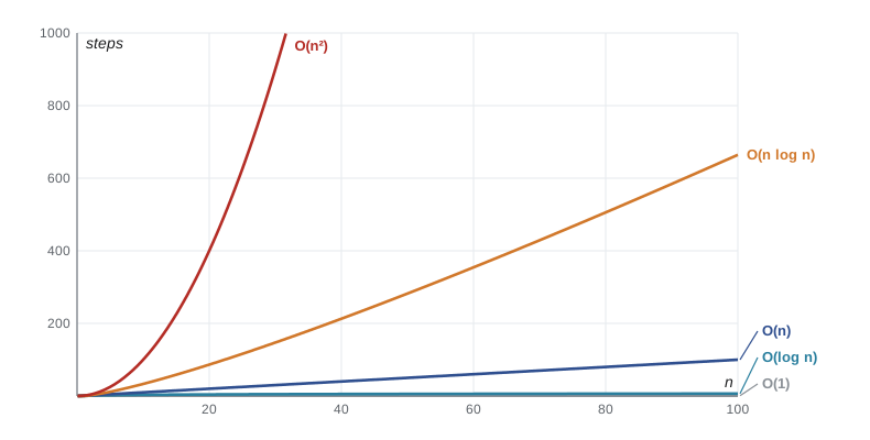
For small inputs, almost any algorithm is fast enough, and the chart shows why the differences surprised the Food Hub only when the data grew. At n = 10 the quadratic algorithm needs 100 steps, which a computer does in well under a microsecond. At n = 10,000 it needs 100,000,000 steps, and that is where a page starts to freeze.
Big-O notation
Big-O notation is the shorthand for these growth rates. Writing that an algorithm is O(n), read as "order n" or "big O of n", means that for large inputs its work grows no faster than some constant times n. The notation keeps only the part of the step count that matters for large n and drops the rest. Two rules do most of the work.
First, drop constant factors. An algorithm that makes 3n + 5 comparisons is O(n), and so is one that makes n ÷ 2. The constant matters in practice, and a careful programmer will still prefer the faster of two O(n) algorithms, but it does not change how the work grows: doubling n doubles the work for both. Constant factors also depend on the machine and the language, which is exactly what Big-O is meant to ignore.
Second, keep only the fastest-growing term. An algorithm that does n² + 100n + 7 steps is O(n²). At n = 10 the 100n term is larger than n², but by n = 1,000 the n² term is ten times larger, and by n = 1,000,000 it is ten thousand times larger. For large inputs, the largest term decides everything.
| Big-O | Name | Doubling n does this to the work | Food Hub example |
|---|---|---|---|
| O(1) | Constant | Nothing | Reading volunteers[0], or looking up a key in a Map |
| O(log n) | Logarithmic | Adds one step | Binary search for a shift time in a sorted list (Lesson 8) |
| O(n) | Linear | Doubles it | Adding up every hamper in the list |
| O(n log n) | Linearithmic | A little more than doubles it | Sorting the volunteer list well (Lesson 7) |
| O(n²) | Quadratic | Multiplies it by four | Comparing every sign-up with every other sign-up |
| O(2ⁿ) | Exponential | Squares it | Trying every possible group of volunteers (Lesson 11) |
Strictly, Big-O describes an upper bound: O(n) promises that the work grows no faster than n. Related notations describe a lower bound (big Omega) and a tight bound (big Theta). In everyday use, including job interviews and code reviews, people say O(n) when they mean the tight bound, and this course does the same.
Reading the Big-O of code
With practice you can find the Big-O of most code by reading it. A few patterns cover most cases. A fixed number of simple statements is O(1). A loop that runs n times, doing O(1) work each time, is O(n). Two loops one after the other are O(n) + O(n), which is still O(n). A loop inside a loop, each running n times, is O(n) × O(n) = O(n²). A loop that halves its range each time is O(log n).
The pattern that causes the most trouble is the hidden loop. A call such as list.includes(x), list.indexOf(x) or list.find(...) looks like one step, but inside it is a loop over the array, so it is O(n). Put one inside another loop and the code is O(n²) even though only one loop is visible.
// The duplicate check from the sign-up form, as it was written in 2026.
function findDuplicatesSlow(emails) {
  let steps = 0;
  const dupes = [];
  for (let i = 0; i < emails.length; i++) {
    for (let j = i + 1; j < emails.length; j++) {
      steps++;
      if (emails[i] === emails[j] && !dupes.includes(emails[i])) dupes.push(emails[i]);
    }
  }
  return { dupes, steps };
}

function makeEmails(n) {
  const out = [];
  for (let i = 0; i < n; i++) out.push('v' + (i % (n - 2)) + '@example.org');
  return out;
}

for (const n of [10, 100, 1000]) {
  const r = findDuplicatesSlow(makeEmails(n));
  console.log('n =', n, 'duplicates:', r.dupes.length, 'comparisons:', r.steps);
}n = 10 duplicates: 2 comparisons: 45 n = 100 duplicates: 2 comparisons: 4950 n = 1000 duplicates: 2 comparisons: 499500
What this code does
The outer loop picks each email and the inner loop compares it with every email after it, so the number of comparisons is n times (n minus 1) divided by 2. Ten times as many emails means about a hundred times as many comparisons, which is quadratic growth. The test data always contains exactly two duplicated addresses so the results are easy to check.
Counting carefully, the inner loop runs n − 1 times for the first email, n − 2 for the second and so on down to 0, which adds up to n(n − 1) ÷ 2. That is ½n² − ½n, and after dropping the constant factor and the smaller term it is O(n²). With 1,000 emails it makes 499,500 comparisons. With the 9,000 sign-ups the Food Hub expects by the end of 2027, it would make about 40 million.
A better algorithm
The slow version compares every pair because it has no memory of what it has already seen. Give it a memory, in the form of a Set, and each email needs only one check: has this address been seen before? Checking whether a Set contains a value takes about the same time however large the Set is, so the whole check becomes one pass through the list.
function findDuplicatesFast(emails) {
  let steps = 0;
  const seen = new Set();
  const dupes = new Set();
  for (const e of emails) {
    steps++;
    if (seen.has(e)) dupes.add(e);
    else seen.add(e);
  }
  return { dupes: [...dupes], steps };
}

function makeEmails(n) {
  const out = [];
  for (let i = 0; i < n; i++) out.push('v' + (i % (n - 2)) + '@example.org');
  return out;
}

for (const n of [10, 100, 1000, 9000]) {
  const r = findDuplicatesFast(makeEmails(n));
  console.log('n =', n, 'duplicates:', r.dupes.length, 'steps:', r.steps);
}n = 10 duplicates: 2 steps: 10 n = 100 duplicates: 2 steps: 100 n = 1000 duplicates: 2 steps: 1000 n = 9000 duplicates: 2 steps: 9000
What this code does
findDuplicatesFast walks through the emails once, remembering each one in the seen Set. An email that is already in the Set is a duplicate. The number of steps equals the number of emails, so the check is linear: 9,000 emails take 9,000 steps instead of about 40 million comparisons.
This is the pattern the whole course keeps returning to. The faster algorithm is not cleverer code inside the loop; it uses a better data structure, and the data structure removes a whole loop. Lesson 5 explains why Set and Map lookups take constant time on average.
Space complexity
Work is not the only cost. The fast duplicate check builds a Set that can hold every email, so its memory use grows with n as well. The space complexity of an algorithm is how its extra memory grows with the input, written in the same Big-O notation. findDuplicatesSlow uses O(1) extra space apart from its result, while findDuplicatesFast uses O(n).
Trading memory for time like this is common and usually worthwhile: storing 9,000 short strings takes well under a megabyte. But space can matter on a cheap tablet, in a Web Worker processing a large file, or in a recursive algorithm whose call stack grows with n, as Lesson 6 shows. A complete analysis states both the time and the space.
Amortized cost
Some operations are usually cheap and occasionally expensive. Adding to the end of a JavaScript array with push is the standard example. The engine keeps some spare room at the end of the array, so most pushes just write into the next free slot. When the room runs out, the engine allocates a larger block, often around twice the size, and copies every element across, which is O(n) for that one push.
Because the block doubles each time, the expensive copies happen rarely, and the total cost of n pushes stays proportional to n. Spread over all of them, each push costs O(1) on average. This is called amortized O(1): not a promise about any single push, but a promise about any long run of them. The simulation below counts the element copies a doubling array would make.
// Simulate an array that doubles its capacity when full.
function simulatePushes(n) {
  let capacity = 1, length = 0, copies = 0;
  for (let i = 0; i < n; i++) {
    if (length === capacity) {
      copies += length;      // copy every element into a bigger block
      capacity *= 2;
    }
    length++;
  }
  return { n, copies, copiesPerPush: (copies / n).toFixed(2) };
}

for (const n of [10, 1000, 1000000]) console.log(simulatePushes(n));{ n: 10, copies: 15, copiesPerPush: "1.50" }
{ n: 1000, copies: 1023, copiesPerPush: "1.02" }
{ n: 1000000, copies: 1048575, copiesPerPush: "1.05" }What this code does
simulatePushes adds n items to an imaginary array that starts with room for one and doubles its room whenever it is full. It counts how many elements have to be copied during the resizes. However large n gets, the copies stay below two per push on average, which is what amortized constant time means.
Real engines use their own growth rules, and the exact factor varies, but any rule that grows by a fixed multiple gives the same amortized result. Lesson 4 meets the opposite case: removing from the front of an array with shift moves every remaining element, which is O(n) every time, with no amortizing to help.
Big-O in practice
Big-O is a tool for decisions, not a score. For the Food Hub's data, a few rules of thumb are enough most of the time. With fewer than about a hundred items, choose the clearest code and stop worrying. With thousands of items, avoid O(n²) work on anything that runs on every key press or every page load. With millions of items, which the Food Hub does not have, even O(n) work may need to move to a Web Worker or the server.
Constant factors and real measurements still matter when two algorithms have the same Big-O, or when n is small. A simple O(n²) sort can beat a complex O(n log n) one on ten items, which is why real sorting functions switch to simple methods for short runs (Lesson 7). The aim of this course is to give you both views: the Big-O that predicts what happens as the data grows, and the counting and measuring that confirm it.
"When you review code," Gareth says, "ask two questions about every loop. How many times does it run when the list is ten times bigger? And is there a hidden loop inside it?" Mira writes the questions on a sticky note and puts it on her monitor.
Try it yourself
Count the comparisons
Lucy wants to know how many pairs of shifts the old clash check compares. The starter function pairCount(n) should return the number of comparisons made by two nested loops where the inner loop starts one after the outer loop, as in findDuplicatesSlow.
Return the result of the formula n × (n − 1) ÷ 2. The program prints the counts for 4, 10 and 300 shifts.
function pairCount(n) {
  return n * n;
}

console.log(pairCount(4));
console.log(pairCount(10));
console.log(pairCount(300));Common mistakes
MistakeAn O(n) algorithm is always faster than an O(n²) one.
InsteadFor large inputs it is. For small inputs constant factors can make the O(n²) one faster, so measure when n is small.
Mistakelist.includes(x) is one step.
InsteadIt is a loop over the array, so it is O(n). Inside another loop it makes the code O(n²).
MistakeBig-O measures time in seconds.
InsteadIt describes how the number of steps grows with the input size, which does not depend on the machine.
MistakeO(2n) is slower than O(n), so it needs its own name.
InsteadConstant factors are dropped: O(2n) is O(n).
MistakeIf the code is fast on today's data, it will stay fast.
InsteadAsk how the work grows. A quadratic algorithm that takes 20 ms on 300 records takes about 2 seconds on 3,000.
Summary and key terms
- An algorithm is a finite, precise list of steps that solves a problem, and a data structure is a way of organizing data so that algorithms can work on it.
- Correctness and termination come before speed.
- Timings depend on the device and the input, so algorithms are compared by how their number of steps grows with the input size n.
- The worst case is the usual measure because it is a guarantee.
- Big-O notation describes growth, dropping constant factors and keeping only the fastest-growing term.
- Common growth rates, from best to worst, are O(1), O(log n), O(n), O(n log n), O(n²) and O(2ⁿ).
- Nested loops multiply, loops in sequence add, and calls such as includes and indexOf hide a loop.
- Replacing a list search with a Set lookup can turn an O(n²) algorithm into an O(n) one.
- Space complexity describes how extra memory grows.
- Amortized O(1), as for push, means a long run of operations averages constant time even if some single operations are expensive.
- algorithm
- A precise, finite list of steps that turns an input into the correct output.
- data structure
- A way of organizing data in memory so that it can be used efficiently, such as an array, Map or tree.
- input size
- The quantity, usually written n, that measures how big the input is, such as the number of records.
- worst case
- The input of a given size that makes an algorithm do the most work.
- Big-O notation
- A way of describing how an algorithm's work grows with n, ignoring constant factors and smaller terms.
- linear time
- Work that grows in proportion to n, written O(n).
- quadratic time
- Work that grows with the square of n, written O(n²), typical of comparing every pair.
- logarithmic time
- Work that grows by one step each time n doubles, written O(log n).
- space complexity
- How the extra memory an algorithm needs grows with the input size.
- amortized cost
- The average cost per operation over a long sequence of operations.
Practice problems
Work each problem on paper first, then reveal the answer to check.
What is the Big-O of a loop over n items that calls list.indexOf on an array of n items each time?
Show answer
O(n²), because indexOf is itself a loop over n items.
Simplify O(5n² + 3n + 20).
Show answer
O(n²): drop the constant factor and keep the fastest-growing term.
Why is the worst case the usual measure?
Show answer
It is a guarantee: the algorithm never does more work than that for an input of that size.
How many comparisons does comparing every pair of 100 items make?
Show answer
100 × 99 ÷ 2 = 4,950.
What does amortized O(1) mean for push?
Show answer
Some pushes copy the whole array, but over many pushes the average cost per push is constant.
Lesson quiz · 5 questions
Score 60% or more to complete this lesson.
Create a free account to save your progress, take quizzes and earn a certificate.