
GEOM-220 · Lesson 8 of 12 · 23 min
Adjusting horizontal networks
Horizontal control networks are the framework for bridges, highways, pipelines, mines and subdivisions. They tie together points that may be hundreds of meters or many kilometers apart, measured by total station, GNSS or both, and their adjusted coordinates become the reference for every stake-out and as-built survey that follows. Adjusting them brings together everything from the earlier lessons: non-linear observation equations for distances and angles, realistic weights for mixed observation types, a datum that fixes position and orientation, and iteration to convergence. This lesson adjusts the core of the bridge control network, two fixed pillars and two new points, and discusses the decisions that a network adjustment forces the surveyor to make.
Kinds of horizontal network
Classical networks were described by what they measured. Triangulation measured angles only, with one or two very carefully measured baselines to give scale; for over a century it was the backbone of national geodetic surveys. Trilateration, which became practical with electronic distance measurement in the 1960s and 1970s, measured distances only. Traversing measured angles and distances along a chain of stations. Today almost every engineering network is a combination: a total station measures directions and distances at each set-up, GNSS fixes some points directly, and the adjustment uses every observation together. The distinction still matters, though, because each observation type controls position in a different way. A distance fixes position along its line, an angle or direction fixes position across its line, and a well-designed network has both, crossing at good angles at every point.
Datum for a horizontal network
A plane network has more freedom than a level network. Its shape is fixed by the observations, but it can be translated in easting and northing and rotated without changing any measured distance or angle. If only angles are measured, it can be scaled as well. The datum must remove each of these freedoms. A network with distances needs at least three constraints: two coordinates of one point and one azimuth, or equivalently two coordinates of one point and one coordinate of another. A network with angles only needs four, with a second fixed point supplying scale as well as orientation.
Holding two well-known points fully fixed, as Leah does here with pillars CR1 and CR2, provides four constraints, one more than the minimum for a network with distances. The adjustment is therefore slightly over-constrained: if the published distance between the pillars disagreed with the new measurements, that disagreement would be forced into the new points. As with level networks, good practice is to run a minimally constrained adjustment first, holding one point and one azimuth, to judge the observations alone, then a constrained adjustment to fit the control and check its consistency.
Preparing the observations
Raw total station data needs several reductions before it enters a horizontal adjustment. Slope distances are reduced to horizontal using the zenith angles, corrected for the instrument's calibrated constant and scale (lesson 4), corrected for atmospheric conditions, and then reduced from the ground to the projection grid. The grid reduction has two parts: an elevation factor, which scales a distance at ground level down to the ellipsoid, and a grid scale factor from the map projection. Their product, the combined factor, is typically within a few hundred parts per million of one.
For the bridge, which lies in the Montana State Plane projection near the Missouri River, the combined factor is about 0.99927, so a 600 m ground distance shrinks by about 0.44 m on the grid. That is two hundred times the measurement precision, and forgetting it is one of the commonest systematic errors in engineering surveys.
Directions observed in several rounds are reduced to mean directions or angles, with the face-left and face-right means removing collimation and trunnion axis errors. Each observation then needs its a priori standard deviation. For distances, Coulee Geomatics uses 2 mm + 2 ppm, which already includes typical centering errors on forced-centering pillars; on tripods over monuments they add a millimeter in quadrature at each end. For angles measured with four sets on a 1″ instrument to targets several hundred meters away, 3″ per angle is a realistic value; on short sights the centering term must be added, as lesson 3 warned.
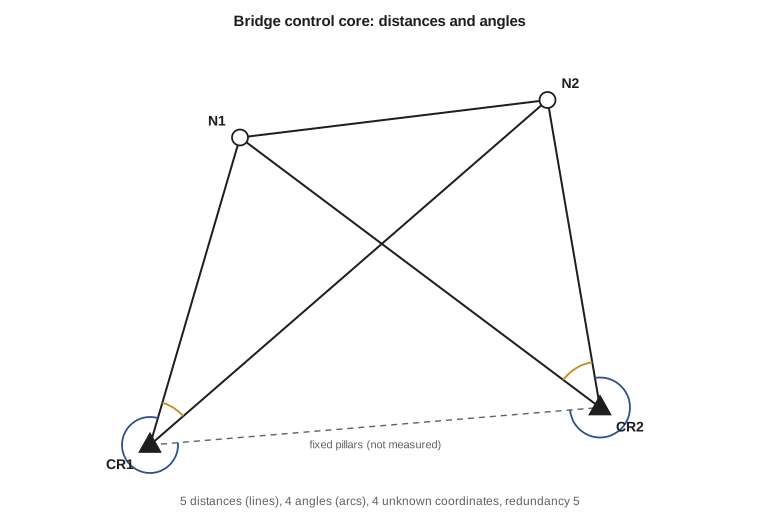
The bridge network
Leah's network has two fixed pillars, CR1 at (5000.000, 5000.000) and CR2 at (5600.000, 5050.000), and two new points, N1 on the east approach and N2 near the planned south abutment. She measured all five distances that do not join the two fixed pillars and four angles: two at CR1 and two at CR2. With four unknown coordinates and nine observations, the redundancy is five.
| Observation | Value | A priori σ |
|---|---|---|
| Distance CR1–N1 | 427.1997 m | 2.9 mm |
| Distance CR1–N2 | 701.7845 m | 3.4 mm |
| Distance CR2–N1 | 599.9995 m | 3.2 mm |
| Distance CR2–N2 | 415.9321 m | 2.8 mm |
| Distance N1–N2 | 413.0357 m | 2.8 mm |
| Angle at CR1, CR2 to N1 | 291°04′38.3″ | 3″ |
| Angle at CR1, N1 to N2 | 32°43′53.6″ | 3″ |
| Angle at CR2, N2 to CR1 | 274°55′31.8″ | 3″ |
| Angle at CR2, N1 to N2 | 43°26′31.8″ | 3″ |
Approximate coordinates come from a quick plot: N1 near (5121, 5408) and N2 near (5528, 5462), each a couple of meters from the truth. Each distance gives an observation equation with the unit-vector derivatives of lesson 5. Each angle is the foresight azimuth minus the backsight azimuth, so its row contains the azimuth derivatives for the foresight point, minus those for the backsight point, and both sets with opposite sign for the occupied station. Where a point is fixed, its columns are simply left out.
Worked problem
Row of the design matrix for an angle
Form the derivative terms for the angle at CR1 from CR2 to N1, using the approximate N1 = (5121.0, 5408.0). CR1 and CR2 are fixed, so only N1's coordinates appear.
Show solution
- \[\Delta E = 121.0, \quad \Delta N = 408.0, \quad d^2 = 121.0^2 + 408.0^2 = 181\,105\ \text{m}^2\]
- \[\frac{\partial \alpha}{\partial E_{N1}} = \frac{\Delta N}{d^2} = \frac{408.0}{181\,105} = 2.253 \times 10^{-3}\ \text{rad/m}\]
- \[\frac{\partial \alpha}{\partial N_{N1}} = -\frac{\Delta E}{d^2} = -\frac{121.0}{181\,105} = -6.68 \times 10^{-4}\ \text{rad/m}\]
- The backsight CR2 is fixed, so it contributes nothing, and the row is \(\begin{bmatrix} 2.253 \times 10^{-3} & -6.68 \times 10^{-4} & 0 & 0 \end{bmatrix}\).
Answer: Moving N1 one meter east changes this angle by 2.25 × 10⁻³ rad, about 465″, so the angle is very sensitive to east-west motion of N1 and much less to north-south motion, as expected for a sight that runs roughly north. In the weighted system the row is divided by the angle's standard deviation in radians, 1.45 × 10⁻⁵, which makes its entries comparable with the distance rows.
def T(A): return [list(r) for r in zip(*A)]
def mul(A, B): return [[sum(a * b for a, b in zip(r, c)) for c in zip(*B)] for r in A]
def inv(A):
    n = len(A); M = [list(map(float, r)) + [1.0 if i == j else 0.0 for j in range(n)] for i, r in enumerate(A)]
    for c in range(n):
        p = max(range(c, n), key=lambda r: abs(M[r][c])); M[c], M[p] = M[p], M[c]
        d = M[c][c]; M[c] = [x / d for x in M[c]]
        for r in range(n):
            if r != c:
                f = M[r][c]; M[r] = [x - f * y for x, y in zip(M[r], M[c])]
    return [r[n:] for r in M]
def diag(v): return [[v[i] if i == j else 0.0 for j in range(len(v))] for i in range(len(v))]
def col(v): return [[x] for x in v]
# Horizontal network: two fixed pillars, two new points, distances and angles
import math

fixed = {'CR1': (5000.000, 5000.000), 'CR2': (5600.000, 5050.000)}
approx = {'N1': (5121.0, 5408.0), 'N2': (5528.0, 5462.0)}
dists = [('CR1', 'N1', 427.1997), ('CR1', 'N2', 701.7845), ('CR2', 'N1', 599.9995),
         ('CR2', 'N2', 415.9321), ('N1', 'N2', 413.0357)]
angles = [  # (at, backsight, foresight, deg, min, sec), clockwise from backsight
    ('CR1', 'CR2', 'N1', 291, 4, 38.3), ('CR1', 'N1', 'N2', 32, 43, 53.6),
    ('CR2', 'N2', 'CR1', 274, 55, 31.8), ('CR2', 'N1', 'N2', 43, 26, 31.8)]
s0 = 1.0                                         # a priori reference sigma (unitless)
RHO = 180 / math.pi * 3600                       # seconds per radian
unk = ['N1', 'N2']
X = dict(fixed); X.update(approx)

def col_of(p, k):                                # column index of coordinate k of p
    return 2 * unk.index(p) + k if p in unk else None

def design():
    A, w, sig = [], [], []
    for a, b, d in dists:
        dE, dN = X[b][0] - X[a][0], X[b][1] - X[a][1]; d0 = math.hypot(dE, dN)
        row = [0.0] * 4
        for p, sgn in ((a, -1), (b, 1)):
            if col_of(p, 0) is not None:
                row[col_of(p, 0)] += sgn * dE / d0; row[col_of(p, 1)] += sgn * dN / d0
        A.append(row); w.append(d - d0); sig.append(0.002 + 2e-6 * d)
    for at, bs, fs, dg, mi, se in angles:
        row = [0.0] * 4; az = {}
        for p, sgn in ((fs, 1), (bs, -1)):
            dE, dN = X[p][0] - X[at][0], X[p][1] - X[at][1]; d2 = dE * dE + dN * dN
            az[p] = math.atan2(dE, dN)
            for q, s2 in ((p, 1), (at, -1)):
                if col_of(q, 0) is not None:
                    row[col_of(q, 0)] += sgn * s2 * dN / d2; row[col_of(q, 1)] -= sgn * s2 * dE / d2
        calc = az[fs] - az[bs]
        obs = math.radians(dg + mi / 60 + se / 3600)
        w.append((obs - calc + math.pi) % (2 * math.pi) - math.pi)
        A.append(row); sig.append(math.radians(3 / 3600))
    return A, w, sig

for it in range(1, 8):
    A, w, sig = design()
    P = diag([(s0 / s) ** 2 for s in sig])       # unitless weights from a priori sigmas
    Qxx = inv(mul(mul(T(A), P), A))
    dx = [r[0] for r in mul(Qxx, mul(mul(T(A), P), col(w)))]
    for i, p in enumerate(unk):
        X[p] = (X[p][0] + dx[2 * i], X[p][1] + dx[2 * i + 1])
    print(f"iteration {it}: largest correction {max(abs(c) for c in dx) * 1000:.2f} mm")
    if max(abs(c) for c in dx) < 1e-5:
        break
A, w, sig = design()                             # at convergence dx = 0, so v = -w
v = [-wi for wi in w]
std = [vi / s for vi, s in zip(v, sig)]
r = len(v) - 4
vtpv = sum(x * x for x in std)
print(f"redundancy r = {r}, vTPv = {vtpv:.2f}, sigma0 = {math.sqrt(vtpv / r):.2f}")
for p in unk:
    i = unk.index(p)
    print(f"{p}: E = {X[p][0]:.4f}  N = {X[p][1]:.4f}  sE = {math.sqrt(Qxx[2*i][2*i]) * 1000:.1f} mm  sN = {math.sqrt(Qxx[2*i+1][2*i+1]) * 1000:.1f} mm")
for (a, b, _), vi in zip(dists, v):
    print(f"  distance {a}-{b:<4} v = {vi * 1000:+6.2f} mm")
for (at, bs, fs, *_), vi in zip(angles, v[len(dists):]):
print(f" angle {bs}-{at}-{fs:<4} v = {vi * RHO:+6.2f} sec")iteration 1: largest correction 2013.30 mm iteration 2: largest correction 13.20 mm iteration 3: largest correction 0.00 mm redundancy r = 5, vTPv = 2.98, sigma0 = 0.77 N1: E = 5119.9999 N = 5409.9994 sE = 2.6 mm sN = 2.5 mm N2: E = 5530.0001 N = 5459.9993 sE = 2.7 mm sN = 2.5 mm distance CR1-N1 v = -0.10 mm distance CR1-N2 v = -1.43 mm distance CR2-N1 v = +0.21 mm distance CR2-N2 v = -0.10 mm distance N1-N2 v = +1.99 mm angle CR2-CR1-N1 v = +0.72 sec angle N1-CR1-N2 v = -3.19 sec angle N2-CR2-CR1 v = -1.27 sec angle N1-CR2-N2 v = -2.89 sec
Interpreting the results
The first iteration moves the points by about two meters, the second by about 13 mm, and the third by less than a hundredth of a millimeter, so the solution has converged. The adjusted coordinates are N1 = (5119.9999, 5409.9994) and N2 = (5530.0001, 5459.9993), each with standard deviations of about 2.5 to 2.7 mm in both coordinates. With five degrees of freedom, \(\mathbf{v}^{\mathsf{T}}\mathbf{P}\mathbf{v} = 2.98\) and \(\hat{\sigma}_0 = 0.77\): the observations fit together slightly better than the a priori standard deviations predicted. Lesson 10 tests whether that is statistically acceptable.
The residuals deserve a look one by one. The largest distance residual is +2.0 mm on N1–N2, about 0.7 of its a priori standard deviation, and the largest angle residual is −3.2″ at CR1, about one standard deviation. Nothing stands out. Two distances, CR1–N1 and CR2–N2, have residuals of only 0.1 mm. That is not necessarily a sign that they were measured exceptionally well. Lesson 10 shows that these two lines have low redundancy numbers: the rest of the network can check them only weakly, so the adjustment leaves them almost unchanged whatever their errors are. Small residuals on weakly checked observations are a warning, not a comfort.
Combining GNSS and terrestrial observations
Many networks now include GNSS baselines alongside total station observations. A baseline gives three coordinate differences in an Earth-centered system, with a full 3 by 3 covariance matrix from the processing. To combine them with plane distances and angles, either the terrestrial observations are reduced to the ellipsoid and the adjustment is done in three-dimensional geodetic coordinates, which is how professional software works, or the GNSS results are first transformed to grid coordinates and introduced as weighted coordinate observations. Either way, the GNSS covariance matrices usually need scaling, since processing software is often optimistic by a factor of two to five, and the relative weights of GNSS and terrestrial observations should be checked by adjusting each group separately first.
For this project the pillars were themselves positioned by static GNSS relative to the NOAA CORS Network, and their NAD83(2011) coordinates were projected to Montana State Plane. The total station network then densifies that control to the accuracy the bridge contractor needs for stake-out.
Common problems in horizontal adjustments
Most failed adjustments trace back to a short list of causes. A station name typed wrongly connects an observation to the wrong point, producing one enormous residual or divergence. An angle reduced with the backsight and foresight swapped gives a residual equal to 360° minus twice the angle. Distances not reduced to grid give a systematic scale error that shows up as positive residuals on every long line when the network is held to control. A wrong instrument or target height affects slope reduction and hence the horizontal distance on steep sights. And a fixed point that has been disturbed forces errors into every new point around it. Theo's rule for Leah is to adjust in stages: first a minimally constrained adjustment of the distances alone, then angles alone, then both together, then the constrained adjustment. Each stage makes it easier to see which observations or which control point is at fault.
A further subtlety is the azimuth and distance between fixed points. When two fixed points are held, the adjustment implicitly assumes that their published separation is exact. If their coordinates came from different surveys or epochs, the implied distance may be wrong by a centimeter or more, and that error will appear in the residuals of every observation near them. Checking a measured distance between the fixed points, where they are intervisible, is a simple safeguard. Here, the pillars were positioned together in one GNSS session and their separation was checked by total station.
Common mistakes
MistakeAdjusting ground distances on a grid.
InsteadApply the combined scale factor so that distances match the grid coordinates.
MistakeHolding all control fixed from the start.
InsteadRun a minimally constrained adjustment first to judge the observations alone.
MistakeUsing the instrument specification alone for short-sight angles.
InsteadAdd centering errors to the a priori standard deviation.
MistakeTrusting small residuals as proof of good observations.
InsteadCheck redundancy numbers; weakly checked observations always have small residuals.
MistakeCombining unscaled GNSS covariances with terrestrial data.
InsteadScale the GNSS covariance matrices from experience or variance component estimates.
Summary and key terms
- Modern horizontal networks combine distances, angles or directions, and often GNSS.
- A network with distances needs at least three datum constraints; with angles only, four.
- Observations must be reduced to the grid, including the combined scale factor.
- Angle rows contain azimuth derivatives for the foresight minus the backsight, and both for the occupied station.
- Iteration converges in a few steps from approximate coordinates good to a few meters.
- Residuals must be read with the redundancy of each observation in mind.
- Adjust in stages and check the consistency of fixed control.
- Triangulation
- A network fixed mainly by measured angles with a few baselines for scale.
- Trilateration
- A network fixed by measured distances.
- Combined scale factor
- The product of the elevation factor and the grid scale factor that reduces ground distances to grid.
- Datum constraint
- A fixed value that removes a freedom of translation, rotation or scale.
- Over-constrained adjustment
- An adjustment holding more control than the minimum required.
- Forced centering
- Mounting instruments and targets interchangeably on the same pillar or tribrach to reduce centering errors.
Practice problems
Work each problem on paper first, then reveal the answer to check.
A network has 3 new points, 14 distances, 10 angles and 2 fixed points. What is the redundancy?
Show answer
r = 24 − 6 = 18.
What is the minimum datum for a plane network of angles only?
Show answer
Four constraints, for example two fixed points.
A 1,200 m ground distance has a combined factor of 0.99960. What is the grid distance?
Show answer
1199.520 m.
An angle's foresight is 300 m due east of the station. What is ∂α/∂N for the foresight?
Show answer
−ΔE/d² = −300/90000 = −0.00333 rad per m.
Two fixed points are 0.015 m further apart in their published coordinates than measured. What will the constrained adjustment show?
Show answer
Residuals and distortion in nearby observations, and a larger σ0 than the minimal adjustment.
Lesson quiz · 5 questions
Score 60% or more to complete this lesson.
Create a free account to save your progress, take quizzes and earn a certificate.