Least squares principle

A survey with no redundancy has a unique answer and no way of checking it. A survey with redundancy has many possible answers, because every subset of the measurements gives a slightly different result, and the surveyor must decide which answer to adopt. Early surveyors used rules of thumb: distribute a traverse misclosure in proportion to leg length, split a triangle's angular misclosure equally. The least squares principle replaces such rules with a single criterion that works for any combination of observations: choose the answer that makes the weighted sum of the squared residuals as small as possible. This lesson explains the principle, why it is the right one for random errors, and how it leads to the normal equations that every adjustment program solves.

Redundancy and the need for a rule

Leah measures three distances along a straight line of pillars: A to B as 150.014 m, B to C as 279.876 m, and A to C as 429.885 m. Two of these are enough to fix the positions of B and C relative to A, so there is one redundant measurement. The three values do not quite agree: A to B plus B to C is 429.890 m, five millimeters more than the direct measurement. Any adjusted solution must change the measurements so that they agree, and there are infinitely many ways to do it. All of the 5 mm could be taken from the direct distance, or from either of the shorter ones, or shared in any proportion.

Each possible solution gives a set of residuals, the corrections \(v_i\) added to the observations to make them consistent. The least squares principle says: pick the solution that minimizes

For the three distances with equal weights, the minimum is reached when the misclosure is shared equally, so each observation is corrected by 1.7 mm in the direction that removes the misclosure. That matches intuition, but the principle also handles cases where intuition gives no clear answer: unequal weights, observations of different kinds, and networks with hundreds of observations and unknowns.

Why squares?

Why minimize the sum of squares rather than, say, the sum of absolute residuals or the largest residual? There are three good reasons, and each one is worth knowing because it also tells us when least squares can mislead.

First, if the errors are normally distributed, the least squares solution is the most probable one: the maximum likelihood estimate. The normal density contains \(\exp(-v^2/2\sigma^2)\), so the probability of a set of independent residuals is proportional to \(\exp(-\tfrac{1}{2}\sum v_i^2/\sigma_i^2)\), which is largest exactly when \(\sum w_i v_i^2\) is smallest. Gauss used this argument in 1809, and Legendre had published the method of least squares in 1805; the famous early success was Gauss's recovery of the asteroid Ceres from a short arc of observations.

Second, even without assuming normal errors, the Gauss-Markov theorem shows that least squares gives the best linear unbiased estimate: among all estimates that are linear in the observations and free of bias, it has the smallest variance. This holds for any error distribution with zero mean and known relative variances.

Third, the arithmetic is linear. Setting the derivatives of a sum of squares to zero gives a set of linear equations, the normal equations, which can be solved directly. Minimizing absolute values or the largest residual needs iterative or linear programming methods, which were impractical in the age of logarithm tables and remain less convenient today.

The same squaring is also the method's weakness. A single blunder of 50 mm contributes 2,500 mm² to the sum, as much as a hundred residuals of 5 mm, so least squares will distort many good observations to reduce one bad one. The blunder's own residual can end up surprisingly small, with its error spread into its neighbors. That is why blunder detection, covered in lesson 10, is an essential companion to least squares rather than an optional extra.

Functional and stochastic models

Every adjustment has two parts. The functional model states the mathematical relationship between the observations and the unknowns: a distance is the difference of two positions along a line, a height difference is the difference of two elevations, a measured distance equals the true distance plus an instrument constant. The stochastic model states the precision of each observation and any correlations, which is to say the weight matrix of lesson 3. A good adjustment needs both. A perfect functional model with unrealistic weights gives wrong precisions and can push errors into the wrong observations; a perfect stochastic model with a missing term in the functional model, such as an uncalibrated prism constant, gives biased results that the statistics may not reveal.

The normal equations

For a linear functional model, the observations \(\boldsymbol{\ell}\) (n of them) are related to the unknowns \(\mathbf{x}\) (u of them) by

where \(\mathbf{A}\) is the n by u design matrix. The residuals are \(\mathbf{v} = \mathbf{A}\mathbf{x} - \boldsymbol{\ell}\). Minimizing \(\mathbf{v}^{\mathsf{T}}\mathbf{P}\mathbf{v}\) by setting its derivative with respect to \(\mathbf{x}\) to zero gives the normal equations and their solution:

The matrix \(\mathbf{N} = \mathbf{A}^{\mathsf{T}}\mathbf{P}\mathbf{A}\) is called the normal matrix. It is square (u by u) and symmetric, and if the unknowns are determinable from the observations it can be inverted. Its inverse \(\mathbf{Q}_{xx} = \mathbf{N}^{-1}\) is the cofactor matrix of the unknowns, and the covariance matrix of the estimated unknowns is \(\hat{\sigma}_0^2\,\mathbf{Q}_{xx}\) (or \(\sigma_0^2\mathbf{Q}_{xx}\) using the a priori value). That result comes from the propagation law of lesson 2: \(\hat{\mathbf{x}}\) is a linear function of \(\boldsymbol{\ell}\) with Jacobian \(\mathbf{N}^{-1}\mathbf{A}^{\mathsf{T}}\mathbf{P}\), and multiplying out \(\mathbf{J}\,\mathbf{P}^{-1}\mathbf{J}^{\mathsf{T}}\) leaves \(\mathbf{N}^{-1}\).

For a single unknown observed directly \(n\) times, \(\mathbf{A}\) is a column of ones and the normal equation reduces to \(\big(\sum w_i\big)\hat{x} = \sum w_i \ell_i\), which is the weighted mean of lesson 3. The weighted mean is the simplest least squares adjustment.

If the normal matrix cannot be inverted, the unknowns are not all determinable from the observations. The commonest cause is a datum defect: a level network with no fixed benchmark, or a horizontal network with no fixed point or orientation. The observations then fix only the shape of the network, not where it sits, and the adjustment needs either fixed control or a minimal constraint. Lessons 7 and 8 deal with this in practice.

Fitting a calibration model

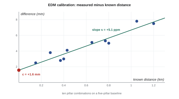
Least squares is also how survey instruments are calibrated, and this gives a neat example with two unknowns. An EDM calibration baseline is a line of concrete pillars whose separations have been determined very precisely. Measuring every pillar-to-pillar combination with the instrument under test, and comparing with the known values, gives a set of differences that should follow the model

where \(c\) is the additive constant, which combines the instrument and prism constants, and \(s\) is the scale error in parts per million. Each combination is one observation equation with two unknowns. Five pillars give ten combinations, eight more than are needed.

The National Geodetic Survey maintains calibration base lines across the United States, including in Montana, with published pillar distances. Coulee Geomatics checks each total station on a calibration base line at least once a year and after any repair, and keeps the results with the instrument's records.

def T(A): return [list(r) for r in zip(*A)]
def mul(A, B): return [[sum(a * b for a, b in zip(r, c)) for c in zip(*B)] for r in A]
def inv(A):
    n = len(A); M = [list(map(float, r)) + [1.0 if i == j else 0.0 for j in range(n)] for i, r in enumerate(A)]
    for c in range(n):
        p = max(range(c, n), key=lambda r: abs(M[r][c])); M[c], M[p] = M[p], M[c]
        d = M[c][c]; M[c] = [x / d for x in M[c]]
        for r in range(n):
            if r != c:
                f = M[r][c]; M[r] = [x - f * y for x, y in zip(M[r], M[c])]
    return [r[n:] for r in M]
def diag(v): return [[v[i] if i == j else 0.0 for j in range(len(v))] for i in range(len(v))]
def col(v): return [[x] for x in v]

# EDM calibration on a five-pillar baseline: fit  measured - known = c + s*D
import math

known = [0.0, 150.012, 429.884, 800.471, 1199.906]     # pillar chainages, m
meas = {(0, 1): 150.0145, (0, 2): 429.8881, (0, 3): 800.4760, (0, 4): 1199.9135,
        (1, 2): 279.8758, (1, 3): 650.4641, (1, 4): 1049.9018,
        (2, 3): 370.5898, (2, 4): 770.0273, (3, 4): 399.4380}
A, l = [], []
for (i, j), m in meas.items():
    D = known[j] - known[i]
    A.append([1.0, D / 1000])          # unknowns: c in mm, s in mm per km (= ppm)
    l.append([(m - D) * 1000])         # observed difference in mm
N = mul(T(A), A)
Qxx = inv(N)
x = mul(Qxx, mul(T(A), l))
v = [mul([a], x)[0][0] - li[0] for a, li in zip(A, l)]
dof = len(l) - 2
s0 = math.sqrt(sum(r * r for r in v) / dof)

c, s = x[0][0], x[1][0]
print(f"additive constant c = {c:+.2f} mm  (sigma {s0 * math.sqrt(Qxx[0][0]):.2f} mm)")
print(f"scale error s      = {s:+.2f} ppm (sigma {s0 * math.sqrt(Qxx[1][1]):.2f} ppm)")
print(f"correlation between c and s = {Qxx[0][1] / math.sqrt(Qxx[0][0] * Qxx[1][1]):.2f}")
print("residuals (mm):", " ".join(f"{r:+.2f}" for r in v))
print(f"a posteriori sigma0 = {s0:.2f} mm with {dof} degrees of freedom")
print(f"correction for a 600 m line: {-(c + s * 0.6):.1f} mm")

additive constant c = +1.57 mm  (sigma 0.40 mm)
scale error s      = +5.11 ppm (sigma 0.58 ppm)
correlation between c and s = -0.88
residuals (mm): -0.16 -0.33 +0.66 +0.20 -0.80 -0.20 -0.86 +0.67 +0.21 +0.61
a posteriori sigma0 = 0.60 mm with 8 degrees of freedom
correction for a 600 m line: -4.6 mm

The fit gives an additive constant of about +1.6 mm and a scale error of about +5.1 ppm, each determined to better than a millimeter or a part per million. A 600 m distance measured with this instrument would therefore read about 4.6 mm long, and the correction of −4.6 mm is larger than the instrument's own random error. The a posteriori standard deviation of 0.6 mm says the residual scatter is small and consistent with good pillar centering.

The output also shows a strong negative correlation, about −0.88, between the constant and the scale. That is typical of straight-line fits when all the abscissas are positive: if the fitted line tilts slightly more steeply, its intercept must drop to stay close to the data. The correlation is harmless as long as both parameters are applied together, but it is a warning against applying a new constant while keeping an old scale factor.

Checks on every solution

Whatever software is used, a few checks catch most arithmetic and modeling errors. The adjusted observations, \(\hat{\boldsymbol{\ell}} = \boldsymbol{\ell} + \mathbf{v}\), must satisfy every geometric condition exactly: the adjusted distances AB and BC must add to the adjusted AC, a level loop must close to zero, the adjusted angles of a triangle must sum to 180° plus the spherical excess. The quantity \(\mathbf{A}^{\mathsf{T}}\mathbf{P}\mathbf{v}\) must be zero to rounding precision, because that is the normal equation rewritten. And \(\mathbf{v}^{\mathsf{T}}\mathbf{P}\mathbf{v}\) computed from the residuals must equal \(\boldsymbol{\ell}^{\mathsf{T}}\mathbf{P}\boldsymbol{\ell} - \hat{\mathbf{x}}^{\mathsf{T}}\mathbf{A}^{\mathsf{T}}\mathbf{P}\boldsymbol{\ell}\). Leah writes these checks into every spreadsheet and script she builds, and Theo will not sign off an adjustment report that does not show the first one.

Linear and non-linear problems

The calibration fit and the collinear distances are linear: each observation is a linear combination of the unknowns, so one solution of the normal equations gives the answer. Most survey problems are not. A distance between two points depends on the square root of the sum of squared coordinate differences; a direction depends on an arctangent. Lesson 5 shows how these are linearized about approximate values of the unknowns and solved by iteration, so that each step is an ordinary linear least squares problem of exactly the form shown here.