Construction layout and curves

Construction layout is where surveying meets the work. Designers produce drawings and models; layout surveyors put the design back on the ground as stakes, nails, paint marks and offsets so that contractors can build it in the right place at the right elevation, and then check that what was built matches the design. Mistakes in layout are expensive, because concrete, pipe and pavement placed in the wrong position may have to be removed. This lesson covers layout control and the principles of staking, building and pipe layout, grade and slope stakes, and the geometry and staking of horizontal circular curves and vertical parabolic curves, using the Coulee Ridge Drive extension.

Coulee Ridge Drive leaves the existing road at station 0+00, runs east on the grade designed in lesson 5, turns right through a circular curve with a radius of 600 ft, and dips through a sag vertical curve at the low point of the site before climbing to meet the subdivision's main entrance. Leah's final task this term is to compute the curve stakeout and the vertical curve elevations, and to check them in the field with Grant.

Layout control and principles

Layout starts from control. Before construction begins, the surveyor sets a network of control points around the site, outside the area that will be disturbed, so that they survive excavation and equipment traffic. Each point is tied to the project coordinate system and benchmarks, and its coordinates and elevation are checked against the design control. Construction stakes are then set from this control by radiation from a total station, by GNSS, or by offsets from reference lines.

Several principles guide layout work. Stakes for important features are set from two independent setups or checked by measuring between them, since a single radiated point has no check. Stakes are usually set on an offset, a fixed distance away from the feature, so that they are not destroyed when the work starts; the marking on each stake gives the offset, the station and the cut or fill. Layout data are computed from the latest approved design, and any discrepancy between the design and the ground is reported to the designer, not silently adjusted. Field books or data files record every stake set, with the date and the design revision used.

Tolerances come from the specifications and the type of work. Anchor bolts and structural steel need millimeters; curbs, sidewalks and pipe inverts need about a centimeter; rough grading may accept a few centimeters. The layout method and instrument should be chosen accordingly: GNSS may be fine for clearing limits and rough grade, while curb, gutter and structures call for a total station.

Buildings, pipes and grade stakes

Buildings are laid out by staking the main corners or column lines from control, then setting offset stakes or batter boards outside the excavation from which strings can be stretched to re-establish the lines after digging. Diagonals of rectangular foundations are measured as a check on squareness: for a rectangle 30 m by 18 m the diagonal must be \(\sqrt{30^2 + 18^2} = 34.986\) m.

Pipes are laid out with offset stakes along a line parallel to the pipe, typically every 15 to 25 m, marked with the station and the cut from the top of the stake to the design invert, the inside bottom of the pipe. In the trench, a pipe laser set to the design grade projects a beam along the pipe axis, and a target in each pipe length is aligned to it. Invert elevations at manholes are computed from the design grade and checked against the profile.

Grade stakes give the cut or fill from the top of the stake, or from a mark on it, to the design elevation. The rod person stands on the stake, the level or total station gives its elevation, and the difference from the design is written on the stake as, for example, C 1.25 for a cut of 1.25 units or F 0.40 for a fill.

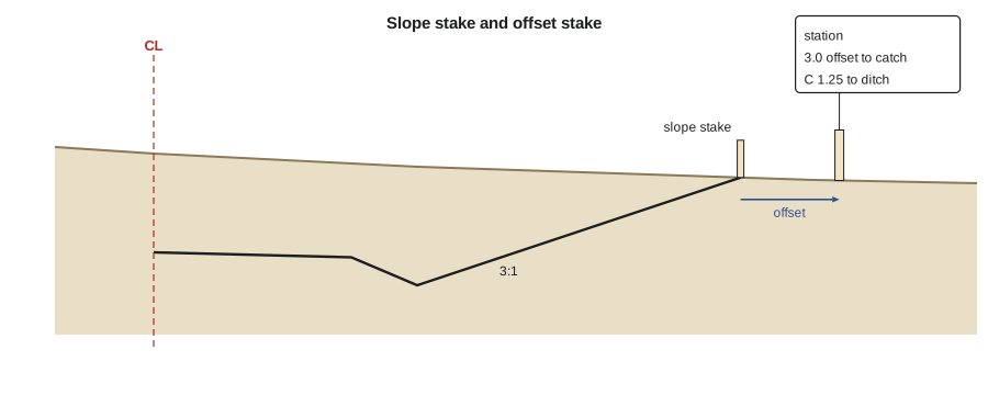
Slope stakes mark the catch points where the design side slopes meet the existing ground, as described in lesson 5. They are found by trial: the surveyor estimates a position, measures the ground elevation and distance from the centerline, computes where the side slope would be at that distance, and moves in or out until the measured ground and the computed slope agree. Modern data collectors do this iteratively in the field, guiding the rod person to the catch point.

Horizontal circular curves

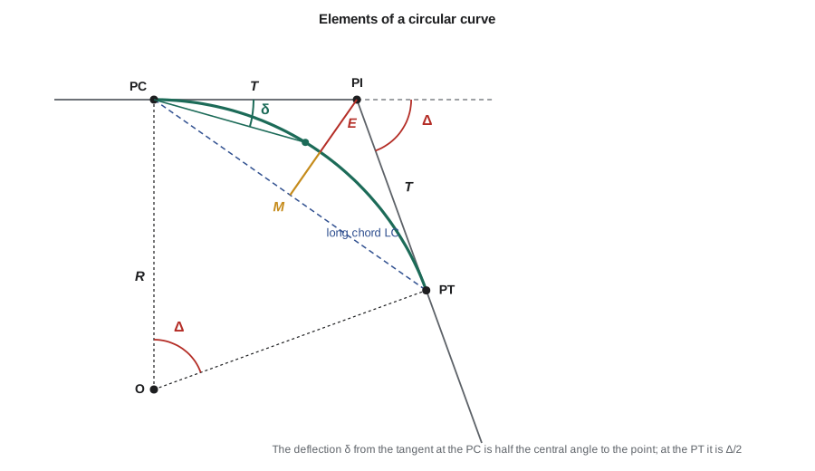
Road and railway alignments consist of straight tangents joined by curves. The simplest is a circular curve of radius \(R\) connecting two tangents that meet at the point of intersection (PI) with an intersection angle \(\Delta\), the change in direction. The curve begins at the point of curvature (PC) and ends at the point of tangency (PT). Its main elements are:

Here \(T\) is the tangent distance from the PI to the PC or PT, \(L\) is the length of the curve along the arc, \(LC\) is the long chord from PC to PT, \(E\) is the external distance from the PI to the middle of the curve and \(M\) is the middle ordinate from the long chord to the middle of the curve. Stationing runs along the tangent to the PC and then along the arc, so:

Note that the PT station is not the PI station plus the tangent distance, because stationing follows the curve, which is shorter than the two tangents.

US highway practice often describes curves by the degree of curve, the central angle subtended by a 100 ft arc, so that \(D = 5729.58/R\) with \(R\) in feet. A curve with a radius of 600 ft is about a 9°33′ curve. Metric projects and many city streets specify the radius directly.

Staking curves by deflection angles

The classical way to stake a curve is from the PC by deflection angles and chords. The deflection angle between the tangent at the PC and the chord to a point on the curve equals half the central angle to that point. For a point at arc distance \(a\) from the PC:

The total station is set on the PC and sighted on the PI with the horizontal circle set to zero; each point is then set by turning its deflection angle and measuring the chord from the PC. The deflection to the PT must equal \(\Delta/2\), which checks the computations. Stakes are usually placed at even stations, so the first point is a short distance from the PC.

Today most curves are staked by coordinates. The design software or the data collector computes the northing and easting of every point on the curve and of its offset stakes, and the crew stakes them from any convenient control point by radiation or with GNSS. The deflection method remains valuable for understanding curve geometry, for checking, and wherever the PC can be occupied conveniently.

Vertical curves

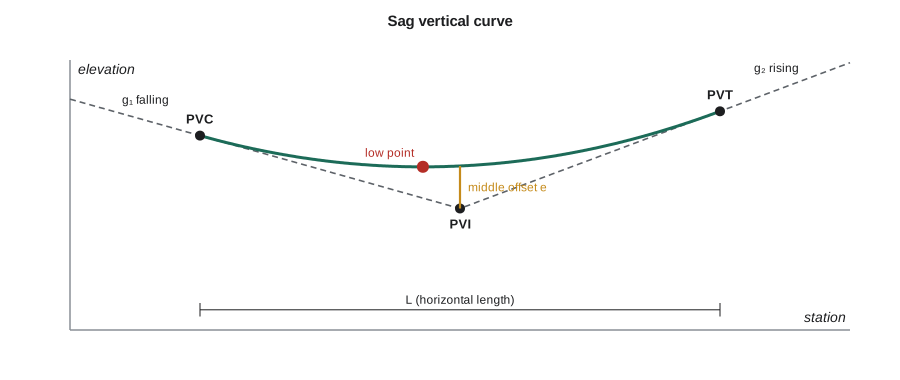
Grades in a profile are joined by vertical curves, which give a smooth change of grade for comfort, safety and drainage. Vertical curves are parabolas rather than circles, because a parabola's rate of change of grade is constant and its elevations are easy to compute. A crest curve joins a rising grade to a falling one; a sag curve joins a falling grade to a rising one. The curve begins at the point of vertical curvature (PVC) and ends at the point of vertical tangency (PVT), and the two grades meet at the point of vertical intersection (PVI). For an equal-tangent curve of horizontal length \(L\), the PVC and PVT are each \(L/2\) from the PVI.

With grades \(g_1\) and \(g_2\) as decimals and \(x\) measured horizontally from the PVC, the elevation on the curve is:

The rate of change of grade is \(r = (g_2 - g_1)/L\). The lowest point of a sag curve, or the highest point of a crest curve, occurs where the grade along the curve is zero, at \(x = -g_1/r\), provided this falls within the curve. The low point matters because that is where a catch basin must be placed to drain the road.

# Horizontal curve stakeout by deflections and coordinates, and a sag vertical curve (feet)
import math

def fmt(deg):
    s = round(deg * 3600); d, s = divmod(s, 3600); m, s = divmod(s, 60)
    return f"{d}°{m:02d}'{s:02d}\""

def sta(x):
    return f"{int(x // 100)}+{x % 100:05.2f}"

PI, R, delta, step = 1353.62, 600.0, 38.4, 50
T = R * math.tan(math.radians(delta / 2)); L = math.pi * R * delta / 180
PC, PT = PI - T, PI - T + L
print(f"T {T:.2f}  L {L:.2f}  PC {sta(PC)}  PT {sta(PT)}  degree of curve {5729.578 / R:.4f}")

# Coordinates: PI at N 16076.12, E 4757.22 ft; back tangent runs east (azimuth 90), curve to the right
NPI, EPI, az_back = 16076.12, 4757.22, 90.0
NPC = NPI - T * math.cos(math.radians(az_back)); EPC = EPI - T * math.sin(math.radians(az_back))
stations = [PC] + [s for s in range(math.ceil(PC / step) * step, int(PT) + 1, step)] + [PT]
for st in stations:
    a = st - PC
    d = math.degrees(a / (2 * R)); c = 2 * R * math.sin(math.radians(d))
    az = math.radians(az_back + d)
    print(f"{sta(st)}  defl {fmt(d):>12}  chord {c:7.2f}  N {NPC + c * math.cos(az):9.2f}  E {EPC + c * math.sin(az):8.2f}")

# Sag vertical curve
pvi, zpvi, g1, g2, Lv = 1840, 2972.20, -0.015, 0.020, 400
pvc, zpvc = pvi - Lv / 2, zpvi - g1 * Lv / 2
r = (g2 - g1) / Lv
for s in range(int(pvc), int(pvi + Lv / 2) + 1, 50):
    x = s - pvc
    print(f"{sta(s)}  curve elevation {zpvc + g1 * x + r / 2 * x * x:.2f}")
x = -g1 / r
print(f"low point {sta(pvc + x)}, elevation {zpvc + g1 * x + r / 2 * x * x:.2f}; middle offset {(g2 - g1) * Lv / 8:.2f} ft")

T 208.94  L 402.12  PC 11+44.68  PT 15+46.80  degree of curve 9.5493
11+44.68  defl     0°00'00"  chord    0.00  N  16076.12  E  4548.28
11+50.00  defl     0°15'15"  chord    5.32  N  16076.10  E  4553.60
12+00.00  defl     2°38'29"  chord   55.30  N  16073.57  E  4603.52
12+50.00  defl     5°01'44"  chord  105.19  N  16066.90  E  4653.06
13+00.00  defl     7°24'58"  chord  154.89  N  16056.13  E  4701.87
13+50.00  defl     9°48'12"  chord  204.32  N  16041.33  E  4749.62
14+00.00  defl    12°11'27"  chord  253.40  N  16022.61  E  4795.96
14+50.00  defl    14°34'41"  chord  302.04  N  16000.10  E  4840.59
15+00.00  defl    16°57'55"  chord  350.15  N  15973.95  E  4883.19
15+46.80  defl    19°12'00"  chord  394.64  N  15946.34  E  4920.97
16+40.00  curve elevation 2975.20
16+90.00  curve elevation 2974.56
17+40.00  curve elevation 2974.14
17+90.00  curve elevation 2973.93
18+40.00  curve elevation 2973.95
18+90.00  curve elevation 2974.18
19+40.00  curve elevation 2974.64
19+90.00  curve elevation 2975.31
20+40.00  curve elevation 2976.20
low point 18+11.43, elevation 2973.91; middle offset 1.75 ft

Machine guidance and modern layout

On many earthwork and paving projects, machine guidance and machine control have replaced much traditional staking. A three-dimensional design surface is loaded into a computer on the dozer, grader or excavator, and GNSS receivers, total stations or lasers on the machine compare the blade or bucket position with the design in real time, either guiding the operator or controlling the hydraulics directly. Surveyors still establish and check the control, build and verify the design surfaces, calibrate the machines, and check the finished work, but the number of grade stakes drops dramatically. The surveyor's role shifts toward data management: making sure every machine, rover and total station uses the same control, coordinate system and design revision.

As-built surveys and checking

Layout is not finished until the work has been checked. Crews survey curb lines, pipe inverts, manhole rims, building corners and finished grades and compare them with the design. Differences beyond tolerance are reported promptly, while they can still be corrected. At the end of the project, the as-built survey records the final positions and elevations for the owner's records and the municipal GIS, closing the loop that began with the control survey in lesson 1.

On the Coulee Ridge project, Leah's last week includes checking the curb at three curve stations against her computed coordinates. All three are within 6 mm in line and 4 mm in grade, well inside the 10 mm tolerance in the specifications, and her stakeout computations become part of the project record.