
GEOM-210 · Lesson 10 of 12 · 24 min
GNSS surveying
Global navigation satellite systems (GNSS) have transformed surveying more than any other technology. A receiver on a pole can now determine its position to a centimeter or two in seconds, without line of sight to any other survey point, day or night and in almost any weather. GNSS is used to establish control, collect topography, stake out designs and guide construction machines. But it is not magic: its accuracy depends on satellite geometry, the environment around the antenna, the method used and the care of the surveyor, and its heights are ellipsoid heights that must be converted to elevations. This lesson explains how GNSS positioning works, its error sources, the main survey methods, and the field practices that make GNSS results reliable.
On the Coulee Ridge project, GNSS was used to position control points CR-1 and CR-5, which fixed the position and orientation of the traverse, and Grant's crew uses real-time kinematic (RTK) GNSS for most topography and rough grading layout in the open parts of the site.
The satellite systems
Four global systems are in operation. The United States' GPS was the first, with about 30 satellites in medium Earth orbit at about 20,200 km altitude. Russia's GLONASS, the European Union's Galileo and China's BeiDou provide similar global coverage, and regional systems, such as Japan's QZSS and India's NavIC, add satellites over their regions. Modern survey receivers track all of them, often more than 40 satellites at once, which greatly improves performance near buildings and trees where some of the sky is blocked.
Each satellite broadcasts signals on several radio frequencies, carrying ranging codes and a navigation message that describes the satellite's orbit and clock. Receivers measure two kinds of observables. Code measurements, also called pseudoranges, compare the received code with a replica to measure the signal travel time, giving a range precise to roughly a meter or a few decimeters. Carrier phase measurements track the phase of the underlying radio wave, whose wavelength is about 19 to 25 cm, and are precise to a few millimeters, but the whole number of wavelengths between satellite and receiver, called the integer ambiguity, is unknown at first and must be resolved.
How a position is computed
A receiver computes its position by trilateration from ranges to satellites whose positions are known from the broadcast orbits. Three ranges would fix a point in three dimensions if the receiver's clock were perfect, but receiver clocks are inexpensive quartz clocks, and an error of one microsecond corresponds to about 300 m of range. The receiver clock error is therefore treated as a fourth unknown, so at least four satellites are needed. With more satellites, the solution is overdetermined and is computed by least squares, which also provides statistics on its quality.
A single receiver using code measurements, called autonomous or standalone positioning, typically achieves a few meters of accuracy, enough for navigation and for finding monuments but not for surveying. Survey accuracy comes from differential methods that compare measurements at two or more receivers, or from precise satellite orbit and clock products that remove most errors, combined with carrier phase measurements.
Error sources
| Error source | Typical size for a single receiver | How surveyors reduce it |
|---|---|---|
| Satellite orbit and clock errors | Decimeters to a meter with broadcast data | Differential methods; precise orbit and clock products |
| Ionospheric delay | Meters, varying with time of day and solar activity | Dual- and multi-frequency receivers; differential methods over short baselines |
| Tropospheric delay | About 2.3 m at the zenith, more at low elevations | Models; differential methods; elevation masks |
| Multipath | Centimeters to meters, from signals reflected off nearby surfaces | Open sites, good antennas, longer observations, avoiding reflective surfaces |
| Antenna phase center variation | Millimeters to centimeters | Calibrated antenna models; consistent antenna orientation |
| Antenna height and centering | Any size, often a blunder | Careful measurement and recording; fixed-height poles and tripods |
| Receiver noise | Millimeters for carrier phase | Quality receivers; averaging |
Many of these errors are spatially correlated: two receivers a few kilometers apart experience nearly the same orbit errors and atmospheric delays. Differencing their measurements cancels most of these common errors, which is the basis of relative positioning. Errors that are local to each antenna, such as multipath, antenna height and centering, do not cancel and must be controlled by field practice.
Satellite geometry and dilution of precision
The accuracy of a GNSS position depends not only on the quality of the range measurements but also on the geometry of the satellites. If the satellites are clustered in one part of the sky, small range errors produce large position errors; if they are spread widely, the position is strong. This effect is expressed by dilution of precision (DOP) factors, which multiply the range error to give the expected position error. PDOP describes three-dimensional position, HDOP horizontal and VDOP vertical position. Values below about 2 indicate good geometry; values above about 4 to 6 call for caution or waiting for better geometry.
Vertical precision is typically about one and a half to two times worse than horizontal, because all satellites are above the horizon, so the vertical component is determined only from one side. Elevation masks, typically 10° to 15°, exclude low satellites whose signals pass through more atmosphere and are more affected by multipath, at the cost of some geometric strength.
Static relative positioning
In static surveys, two or more receivers record carrier phase data simultaneously for a session, usually from about 20 minutes to several hours depending on the distance between receivers, called the baseline length, and the accuracy required. The data are processed afterward to compute the three-dimensional vector between each pair of receivers. Networks of baselines, with redundant connections and ties to several published control points, are then adjusted by least squares. Static GNSS is the most accurate surveying method in common use, routinely achieving a few millimeters plus about 1 part per million of the baseline length, and it is used for primary control networks, deformation monitoring and geodetic work.
An alternative to running one's own base receiver is to process a single receiver's static data against permanent reference stations. The National Geodetic Survey's OPUS service accepts a file of observations, processes it against nearby CORS, and returns NAD83(2011) and ITRF coordinates, typically good to a centimeter or two for a few hours of dual-frequency data. Grant used both a base receiver on an NGS control monument and OPUS to position CR-1, and compared the results.
Real-time kinematic positioning
Real-time kinematic (RTK) GNSS uses a base receiver on a point of known coordinates and a rover receiver that moves between points. The base transmits its measurements or corrections to the rover by radio or over a cellular data connection, and the rover computes its position relative to the base in real time. Once the rover has resolved the integer ambiguities, a state called a fixed solution, it typically achieves about 1 to 2 cm horizontally and 2 to 3 cm vertically within about 10 km of the base, with accuracy degrading by roughly 1 part per million of the baseline length. A float solution, in which ambiguities are not yet resolved, may be wrong by decimeters and must never be used for surveying.
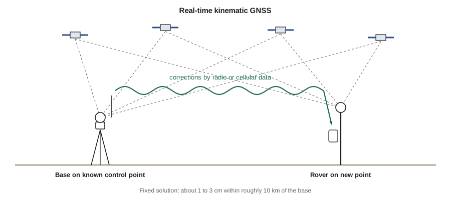
Network RTK replaces the single base with a network of permanent reference stations operated by governments or commercial providers. A central server models the errors across the region and sends corrections suitable for the rover's location, often in the form of a virtual reference station near the rover. Network RTK saves setting up a base and gives consistent coordinates across a region, provided the network's coordinates are tied to the official reference system. Surveyors must know which datum and realization the network uses, because the rover's coordinates inherit them.
Worked problem
Expected RTK precision
A rover is 8 km from the RTK base. The manufacturer's specification is ±(8 mm + 1 ppm) horizontally and ±(15 mm + 1 ppm) vertically. What precision can be expected, and how does that compare with a 5 mm requirement for drainage benchmarks?
Show solution
- Horizontal: \(8 + 1 \times 8 = 16\) mm.
- Vertical: \(15 + 1 \times 8 = 23\) mm.
- These are one-standard-deviation values under good conditions; at 95 percent confidence they are roughly doubled.
Answer: Expect about 16 mm horizontally and 23 mm vertically, or about 3 to 5 cm at 95 percent confidence. That is fine for topography and rough grading but far from the 5 mm needed for drainage benchmarks, which is why BM-8 was established by leveling.
Precise point positioning (PPP) uses precise satellite orbits and clocks from global networks, delivered over the internet or by satellite, to position a single receiver without a local base. Real-time PPP services now reach a few centimeters after a convergence period of several minutes, and hybrid methods called PPP-RTK shorten that convergence. They are especially useful in remote areas without nearby reference stations.
Computing dilution of precision
DOP values come from the geometry matrix of the least squares solution. Each row describes the direction from the receiver to one satellite, in terms of its azimuth and elevation, plus a column for the receiver clock. The program below computes PDOP, HDOP and VDOP for a good spread of satellites and for satellites bunched overhead, showing why geometry matters.
# Dilution of precision from satellite azimuths and elevations
import math

def dops(sats):
    A = []
    for az, el in sats:
        a, e = math.radians(az), math.radians(el)
        A.append([-math.cos(e) * math.sin(a), -math.cos(e) * math.cos(a), -math.sin(e), 1.0])
    N = [[sum(r[i] * r[j] for r in A) for j in range(4)] for i in range(4)]
    M = [N[i][:] + [1.0 if i == j else 0.0 for j in range(4)] for i in range(4)]
    for c in range(4):                       # Gauss-Jordan inverse
        p = max(range(c, 4), key=lambda r: abs(M[r][c])); M[c], M[p] = M[p], M[c]
        piv = M[c][c]; M[c] = [x / piv for x in M[c]]
        for r in range(4):
            if r != c:
                f = M[r][c]; M[r] = [x - f * y for x, y in zip(M[r], M[c])]
    Q = [row[4:] for row in M]
    return (math.sqrt(Q[0][0] + Q[1][1] + Q[2][2]), math.sqrt(Q[0][0] + Q[1][1]), math.sqrt(Q[2][2]))

spread = [(0, 75), (45, 30), (130, 40), (220, 25), (300, 35), (170, 15), (80, 60)]
bunched = [(0, 80), (30, 70), (60, 75), (90, 65)]
for name, s in (("well spread, 7 satellites", spread), ("bunched overhead, 4 satellites", bunched)):
    p, h, v = dops(s)
    print(f"{name}: PDOP {p:.1f}, HDOP {h:.1f}, VDOP {v:.1f}")

sigma_range = 0.005   # carrier-phase range error after differencing, m
p, h, v = dops(spread)
print(f"expected horizontal error {h * sigma_range * 1000:.1f} mm, vertical {v * sigma_range * 1000:.1f} mm")

# RTK specification at increasing baseline length
for km in (1, 5, 10, 20):
print(f"{km:2d} km: H {8 + km:.0f} mm, V {15 + km:.0f} mm (1 sigma)")well spread, 7 satellites: PDOP 2.3, HDOP 1.1, VDOP 2.0 bunched overhead, 4 satellites: PDOP 46.4, HDOP 12.8, VDOP 44.6 expected horizontal error 5.5 mm, vertical 10.0 mm 1 km: H 9 mm, V 16 mm (1 sigma) 5 km: H 13 mm, V 20 mm (1 sigma) 10 km: H 18 mm, V 25 mm (1 sigma) 20 km: H 28 mm, V 35 mm (1 sigma)
Field practice for reliable GNSS
The difference between a good and a bad GNSS survey is usually field practice, not equipment.
- Check in on known control at the start of every session and whenever the base or network changes: occupy a known point and compare the measured coordinates with the published values. A check that disagrees by more than the expected precision means something is wrong with the base setup, the coordinate system, the antenna height or the network settings.
- Measure and record antenna heights carefully. Know whether the height is measured to the antenna reference point or to a mark on the antenna, vertically or along a slant, and enter it correctly. A wrong antenna height is the most common GNSS blunder and shifts every elevation by the same amount.
- Avoid obstructions and reflectors. Trees, buildings, vehicles and fences block or reflect signals. A point next to a building may give a fixed solution that is wrong by several centimeters because of multipath.
- Use redundancy. Important points should be occupied twice, at times far enough apart, typically at least an hour or two, for the satellite geometry to change, and with a fresh initialization. Agreement between the two occupations is strong evidence that the positions are right.
- Watch the quality indicators. Accept only fixed solutions, check the reported precisions and DOP, and be suspicious of a solution that fixes very quickly in poor conditions.
- Document the coordinate system. Record the datum, realization, epoch, geoid model, projection and units used by the base, the network and the data collector.
GNSS heights
GNSS measures ellipsoid heights, which are converted to elevations with a geoid model as explained in lesson 9. With RTK and a modern geoid model, elevations are typically good to a few centimeters, which is suitable for topography, earthwork and rough grading. For flat drainage design, floor slabs and benchmarks, differential leveling remains the method of choice, and GNSS elevations should be checked against local benchmarks. A useful technique on construction sites is a site calibration or localization, in which RTK positions are compared with several local control points and a small transformation is computed so that GNSS results match the project's control. It must be done with well-distributed control points and documented carefully, because a poor localization distorts everything measured afterward.
Limitations and vulnerabilities
GNSS signals are extremely weak by the time they reach the Earth, so they are easily blocked and vulnerable to interference. Under tree canopy, in urban canyons, in tunnels and indoors, GNSS may be unavailable or unreliable, and total stations remain essential. Strong solar activity can disturb the ionosphere and degrade RTK for hours. Deliberate or accidental radio interference, called jamming, and false signals, called spoofing, are growing concerns for machine control and other critical uses. Surveyors therefore treat GNSS as one tool among several, combining it with total stations and levels and always checking on known points.
Common mistakes
MistakeAccepting a float solution because the coordinates look reasonable.
InsteadUse only fixed solutions for surveying, and verify them with check shots or repeat occupations.
MistakeEntering the antenna height to the wrong reference point or as a slant height.
InsteadRecord exactly what was measured and how, and enter it to match the receiver’s settings.
MistakeUsing GNSS ellipsoid heights directly as elevations.
InsteadApply the geoid model for the vertical datum, and check against local benchmarks.
MistakeAssuming a real-time network uses the same datum as the project.
InsteadConfirm the network’s datum, realization and epoch, and check in on known control.
Summary and key terms
- GPS, GLONASS, Galileo and BeiDou provide global coverage; modern receivers track all of them.
- Code measurements give meter-level ranges; carrier phase gives millimeter precision once integer ambiguities are resolved.
- At least four satellites are needed because the receiver clock error is an unknown; DOP describes the strength of the geometry.
- Static relative positioning is the most accurate method; RTK gives 1 to 3 cm in real time; PPP needs no local base.
- Field practice controls most GNSS errors: check shots, antenna heights, open sites, redundancy and quality indicators.
- GNSS heights are ellipsoid heights; elevations need a geoid model, and leveling is still used where millimeters matter.
- GNSS
- Global navigation satellite systems, including GPS, GLONASS, Galileo and BeiDou.
- Pseudorange
- A range measured from the travel time of a satellite code signal, including the receiver clock error.
- Carrier phase
- A precise measurement of the phase of a satellite signal’s carrier wave.
- Integer ambiguity
- The unknown whole number of carrier wavelengths between satellite and receiver.
- DOP
- Dilution of precision, a factor describing how satellite geometry affects position accuracy.
- RTK
- Real-time kinematic positioning using corrections from a base or network to give centimeter positions in real time.
- Fixed solution
- An RTK solution in which the integer ambiguities have been resolved.
- Multipath
- Errors caused by satellite signals reaching the antenna after reflecting off nearby surfaces.
Practice problems
Work each problem on paper first, then reveal the answer to check.
Why does a GNSS receiver need signals from at least four satellites?
Show answer
To solve for three coordinates and the receiver clock error.
An RTK specification is ±(10 mm + 1 ppm) horizontally. What is the expected precision at 15 km?
Show answer
25 mm.
If the range error is 5 mm and HDOP is 1.2, estimate the horizontal error.
Show answer
About 6 mm.
Why is vertical GNSS precision usually worse than horizontal?
Show answer
All satellites are above the horizon, so the vertical component is determined from one side only.
How can a wrong antenna height be detected?
Show answer
By checking in on a known control point, where every measured elevation would be off by the same amount.
Name two situations where a total station is preferable to GNSS.
Show answer
Under heavy tree canopy or next to tall buildings, and indoors or in tunnels; also for millimeter-level layout.
Lesson quiz · 5 questions
Score 60% or more to complete this lesson.
Create a free account to save your progress, take quizzes and earn a certificate.