Power amplifiers

The TLR-1 cabinet transmitted 14 dBm, then 20 dBm after the ELE-350 design review, straight from its transceiver chip. TLR-2 raises the cabinet's telemetry power to 27 dBm, half a watt, so that cabinet-to-cabinet links between widely spaced intersections keep a large margin even through trees and passing trucks. The rules for 902–928 MHz frequency-hopping systems allow up to 30 dBm with antennas of up to 6 dBi, as ELE-350 found, so 27 dBm leaves room. Half a watt is beyond what the transceiver can provide, and Priya must add an external power amplifier (PA). A PA is the part of a radio that turns supply power into radio-frequency power, and its efficiency, linearity and spectral purity decide how much heat the cabinet unit must shed, how far the signal reaches and whether the product can be certified.

Output power and the load line

A transistor delivering power behaves very differently from a small-signal amplifier. Its output voltage swings almost from the knee voltage V_k, below which the transistor stops behaving as a current source, up to nearly twice the supply voltage, and its current swings from near zero to a peak value. The load resistance that lets the transistor use the full voltage swing at the required output power is the optimum load, or load line.

For 27 dBm (501 mW) from the cabinet's 3.6 V rail with a 0.3 V knee, R_opt is about 10.9 Ω. This is the impedance the matching network must present to the transistor, and it is not the conjugate of the transistor's output impedance. Matching for maximum small-signal gain would make the voltage swing too large and drive the transistor into clipping at a lower output power; matching to the load line lets it deliver its full power. Real devices have output capacitance and package parasitics, and the optimum load is found more precisely by load-pull: a tuner presents a range of impedances to the transistor while its output power and efficiency are measured, and the designer chooses the impedance that best balances the two. The manufacturer of Priya's PA transistor publishes load-pull contours, and the 12 Ω target used for the Pi network in lesson 3 comes from them.

import math

# Cabinet sub-GHz power amplifier for TLR-2: 27 dBm at 915 MHz from a 3.6 V supply
def dbm_w(p): return 10**(p/10)/1000
Vdd, Vk, Pout_dbm = 3.6, 0.3, 27.0
P = dbm_w(Pout_dbm)
Ropt = (Vdd - Vk)**2/(2*P)
print(f"load line: Ropt = (Vdd - Vk)^2 / 2P = {Ropt:.2f} ohm for {P*1000:.0f} mW")

# Ideal drain efficiency versus output back-off for class A and class B
print("back-off  class A  class B")
for bo in (0, 3, 6, 10):
    r = 10**(-bo/20)                   # amplitude ratio
    print(f"  {bo:2d} dB   {50*r*r:5.1f} %  {78.5*r:5.1f} %")

# Power-added efficiency of a real class AB stage
Pin_dbm, Idc = 13.0, 0.36           # drive and measured supply current at full power
Pdc = Vdd*Idc; pae = (P - dbm_w(Pin_dbm))/Pdc
print(f"DC input {Pdc:.2f} W, drain efficiency {P/Pdc*100:.1f} %, PAE {pae*100:.1f} %")

# Two-tone intermodulation from OIP3, and the adjacent-channel effect
oip3 = 38.0
for po in (27, 24, 21):              # output power per tone, dBm
    im3 = 3*po - 2*oip3
    print(f"  {po} dBm per tone: IM3 product {im3:5.1f} dBm  ({po - im3:4.1f} dBc)")

# Harmonic budget against the general field-strength limit above 960 MHz
# 500 microvolts per m at 3 m (54 dBuV/m) corresponds to an EIRP of about 54 - 95.2 = -41.2 dBm
limit_eirp = 54 - 95.2
for n, hdbc, gain in ((2, -18, 0.0), (3, -25, 1.0), (4, -38, 0.0)):
    native = Pout_dbm + hdbc
    need = native + gain - (limit_eirp - 6)      # 6 dB margin
    print(f"harmonic {n} at {n*0.915:.3f} GHz: {native:5.1f} dBm from the PA, filter must give {need:4.1f} dB")

# How much of that the Pi matching network (lesson 3: 17.2 pF, 3.64 nH, 10.4 pF) already provides
def pi_gain(f):
    w = 2*math.pi*f; z = 1/(1j*w*10.4e-12)
    zl = 1/(1/50 + 1/z)                      # C2 in parallel with the 50-ohm load
    zs = 1j*w*3.64e-9 + zl                   # series L
    zp = 1/(1/zs + 1j*w*17.2e-12)            # C1 at the PA side
    p_load = abs(zl/zs)**2/50                # power into 50 ohm for 1 V at the transistor node
    return zp, p_load
z0, p0 = pi_gain(915e6)
for n in (2, 3, 4):
    zp, p = pi_gain(n*915e6)
    print(f"Pi match at harmonic {n}: about {10*math.log10(p0/p):4.1f} dB more rejection than at 915 MHz (same swing at the transistor)")

load line: Ropt = (Vdd - Vk)^2 / 2P = 10.86 ohm for 501 mW
back-off  class A  class B
   0 dB    50.0 %   78.5 %
   3 dB    25.1 %   55.6 %
   6 dB    12.6 %   39.3 %
  10 dB     5.0 %   24.8 %
DC input 1.30 W, drain efficiency 38.7 %, PAE 37.1 %
  27 dBm per tone: IM3 product   5.0 dBm  (22.0 dBc)
  24 dBm per tone: IM3 product  -4.0 dBm  (28.0 dBc)
  21 dBm per tone: IM3 product -13.0 dBm  (34.0 dBc)
harmonic 2 at 1.830 GHz:   9.0 dBm from the PA, filter must give 56.2 dB
harmonic 3 at 2.745 GHz:   2.0 dBm from the PA, filter must give 50.2 dB
harmonic 4 at 3.660 GHz: -11.0 dBm from the PA, filter must give 36.2 dB
Pi match at harmonic 2: about 18.5 dB more rejection than at 915 MHz (same swing at the transistor)
Pi match at harmonic 3: about 26.5 dB more rejection than at 915 MHz (same swing at the transistor)
Pi match at harmonic 4: about 31.8 dB more rejection than at 915 MHz (same swing at the transistor)

Amplifier classes and efficiency

Power amplifiers are grouped into classes by how the transistor conducts over each cycle. In class A the transistor conducts for the whole cycle, biased at half its peak current; it is the most linear and the least efficient, with a theoretical drain (or collector) efficiency of 50 % at full output. In class B it conducts for half the cycle, in class AB for somewhat more than half, and in class C for less. Reducing the conduction angle raises the efficiency, to 78.5 % for ideal class B, but produces more harmonics and, in class C, a gain that depends on the drive level.

Switching amplifiers go further. In classes D, E and F the transistor is driven as a switch, nearly fully on or fully off, and the output network shapes the voltage and current waveforms so that they do not overlap. With ideal parts the efficiency approaches 100 %; in practice, at 915 MHz, well-designed class E and F amplifiers reach 60 to 75 %. They cannot reproduce amplitude variations at all, so they suit only constant-envelope signals unless combined with supply modulation.

Efficiency at full power is only half the story, because many signals do not stay at full power. The program shows that an ideal class A amplifier's efficiency falls in proportion to its output power: 25 % at 3 dB back-off and 5 % at 10 dB. Class B falls in proportion to output amplitude, more gently: 55.6 % at 3 dB and 24.8 % at 10 dB.

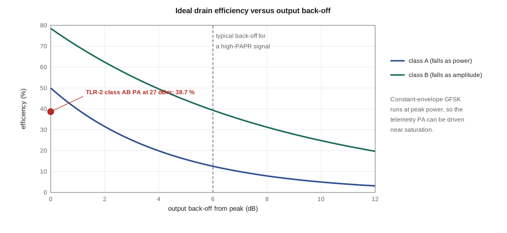
The TLR-2 telemetry signal is GFSK, whose envelope is constant: the amplifier can run at its peak power on every transmission, which is the best case for efficiency. Priya chooses a class AB amplifier driven close to saturation. At 27 dBm out with 13 dBm of drive, it draws 0.36 A from 3.6 V. Its drain efficiency is 38.7 % and its power-added efficiency (PAE), which subtracts the drive power, is 37.1 %.

The difference between the 1.30 W drawn from the supply and the 0.5 W delivered, about 0.8 W, becomes heat in the transistor while it transmits. The cabinet unit transmits about 3 % of the time, so the average heat is small, but the transistor must handle the peak: its package needs a thermal path through many vias to the ground plane, and Priya checks the junction temperature at the 60 °C maximum cabinet air temperature with the method of ELE-340.

Linearity: compression, intermodulation and spectral regrowth

An amplifier driven hard enough compresses: its gain falls as the output approaches saturation. The 1 dB compression point P1dB is the output power at which the gain has fallen 1 dB below its small-signal value. Compression changes amplitude (AM-to-AM conversion) and usually phase as well (AM-to-PM conversion). For a constant-envelope signal neither matters much, because the envelope never changes; for any signal whose envelope varies, compression distorts it.

The cellular module's transmitter is the contrast. LTE uplinks use single-carrier frequency-division multiple access, a form of modulation whose envelope varies with a peak-to-average power ratio (PAPR) of several decibels, and QPSK or 16-QAM symbols whose amplitudes carry information. Its amplifier must run backed off from saturation, and its efficiency is correspondingly lower, which is one reason the cellular module draws more current than the telemetry radio for a similar output power. Lesson 10 returns to this when comparing energy per message.

Third-order intermodulation measures linearity with two tones. With two equal tones at f₁ and f₂, a nonlinear amplifier produces products at 2f₁ − f₂ and 2f₂ − f₁ that grow three times as fast as the tones, in decibels, and the output third-order intercept OIP3 is where they would meet. The program uses OIP3 = 38 dBm for the PA: at 27 dBm per tone the products are only 22 dB below the tones; at 21 dBm per tone, 34 dB below. For a modulated signal the equivalent effect is spectral regrowth: intermodulation among the signal's own spectral components spreads energy into the adjacent channels. It is measured as the adjacent-channel leakage ratio (ACLR) or adjacent-channel power ratio (ACPR), the power in a neighboring channel relative to the wanted channel, and cellular standards set limits on it. The module maker handles this for the cellular radio; for the GFSK telemetry, spectral regrowth is small because the envelope is constant.

Harmonics and spurious emissions

Driven near saturation, the class AB amplifier generates strong harmonics: Priya's data sheet suggests the second harmonic about 18 dB and the third about 25 dB below the carrier before any filtering. Radio rules limit everything a transmitter radiates outside its authorized band. For frequency-hopping systems in 902–928 MHz, emissions outside the band must be at least 20 dB below the in-band level, and emissions falling in restricted bands must meet the general field-strength limits, which above 960 MHz are 500 µV/m at 3 m, 54 dBµV/m. The rule of thumb that converts field strength at 3 m into equivalent isotropically radiated power (EIRP) is E(dBµV/m) ≈ EIRP(dBm) + 95.2, so 54 dBµV/m corresponds to about −41 dBm EIRP.

Cedarline's design rule is stricter than the regulations require: every harmonic of the telemetry transmitter must meet the restricted-band limit with 6 dB of margin, whether or not it falls in a restricted band, because a harmonic that passes the relative limit on the bench may fall in a restricted band when the hopping channel changes, and because the same product must pass in both Canada and the United States. The program turns that rule into a filter specification: the harmonic filter must provide about 56 dB at the second harmonic, 50 dB at the third and 36 dB at the fourth.

The lesson 4 Chebyshev filter gives about 30, 50 and 63 dB at those frequencies. The Pi output match from lesson 3, because of its loaded Q of 3, adds about 18.5 dB more rejection at the second harmonic than at the carrier, 26.5 dB at the third and 31.8 dB at the fourth, for the same voltage swing at the transistor. Together they give about 49 dB at the second harmonic, 7 dB short of the target, and comfortable margins at the third and fourth. The 1830 MHz trap that Priya added in lesson 4 closes the gap: Leo measures 22 dB of additional rejection from it on the fixture. Lesson 12 checks the final numbers against radiated measurements.

Ruggedness, protection and power control

A power amplifier must survive the worst load it will ever see. A broken antenna cable, water in a connector or a technician disconnecting the antenna during a transmission can present an open or short circuit, reflecting all the power back. The reflected wave adds to the forward wave at the transistor, raising the peak voltage, and can destroy it. Data sheets state ruggedness as the VSWR, often 10:1 at all phase angles, that the device survives at a given supply and drive. Priya adds a directional coupler and detector after the harmonic filter so that the microcontroller can measure forward and reflected power, turn the power down if the reflected power exceeds a threshold, and log an antenna fault for the maintenance app. The same detector lets the firmware hold the output at 27 dBm as the supply and temperature vary.

The cabinet unit also needs to reduce power on short links. Two cabinets 150 m apart do not need half a watt, and transmitting less reduces interference to neighboring systems, a courtesy the rules encourage. TLR-2 adjusts its power so that the received signal strength reported by the other cabinet stays about 30 dB above sensitivity, a margin chosen to cover fading.