
ELE-455 · Lesson 2 of 12 · 25 min
S-parameters and network analysis
Leo's first job on TLR-2 is to measure the SAW filter that Amara has chosen for the cabinet receiver. At low frequencies he would measure a component with a voltmeter and an ammeter, or with an impedance bridge. At 915 MHz neither works. Open and short circuits, which low-frequency measurements rely on, are hard to make: a short has inductance, an open radiates and has capacitance, and the connecting wires are a significant fraction of a wavelength, so the voltage and current at the instrument are not those at the device. Radio-frequency engineers describe and measure components instead with scattering parameters, which relate waves traveling into and out of a device rather than voltages and currents at its terminals.
This lesson defines scattering parameters, shows how they relate to impedance and to the quantities on data sheets, introduces the vector network analyzer that measures them, and explains calibration and de-embedding, the techniques that remove the effects of cables, connectors and test fixtures. Everything later in the course, from matching networks to amplifier stability, is expressed in S-parameters.
Waves instead of voltages
ELE-360 showed that on a transmission line of characteristic impedance Z₀ the voltage at any point is the sum of a forward and a reflected wave. Scattering parameters build on that picture. At each port of a device we define an incident wave aₙ and a reflected wave bₙ, normalized so that their squared magnitudes are powers: |a₁|²/2 is the power flowing into port 1 and |b₁|²/2 the power flowing out, when the port is connected to a line of impedance Z₀, almost always 50 Ω.
For a linear two-port, the outgoing waves are linear combinations of the incoming ones, and the coefficients form the scattering matrix.
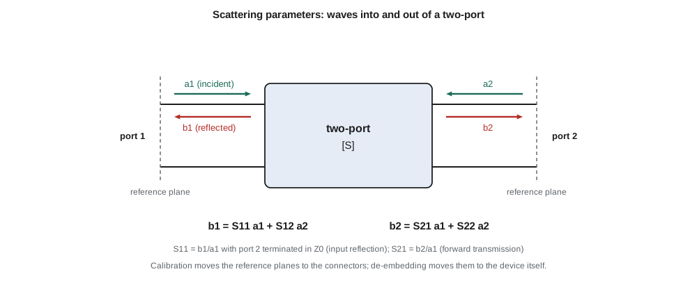
Each parameter has a direct physical meaning when the other port is terminated in Z₀, so that its incident wave is zero. S₁₁ is the input reflection coefficient, the Γ of ELE-360 seen looking into port 1. S₂₁ is the forward transmission coefficient: its magnitude squared is the power gain of an amplifier, or the fraction of power a filter passes. S₁₂ is the reverse transmission, which describes how much of a signal at the output leaks back to the input, and S₂₂ is the output reflection coefficient. All four are complex numbers that vary with frequency, and a data sheet gives them as magnitude and angle at a list of frequencies, usually in a Touchstone file that circuit simulators read directly.
The quantities engineers quote
Engineers rarely quote S-parameters directly. They quote quantities derived from them, in decibels.
| Quantity | Definition | Typical TLR-2 value |
|---|---|---|
| Return loss | −20 log₁₀|S₁₁| | Antenna port better than 10 dB, filter ports better than 15 dB |
| Insertion loss | −20 log₁₀|S₂₁| for a passive part | SAW filter 1.5 dB |
| Gain | 20 log₁₀|S₂₁| for an amplifier | LNA 15 to 17 dB |
| Isolation (reverse) | −20 log₁₀|S₁₂| | LNA about 25 dB |
| VSWR | (1 + |S₁₁|)/(1 − |S₁₁|) | Antenna under 2:1 in band |
| Mismatch loss | −10 log₁₀(1 − |S₁₁|²) | 0.5 dB at VSWR 2:1 |
Return loss and VSWR describe the same thing in two ways, and both appeared in ELE-360. Mismatch loss tells the designer how much power is lost to reflection, which is surprisingly little at moderate mismatch: a VSWR of 2:1, which looks bad on a Smith chart, loses only 0.5 dB. Insertion loss of a passive part includes both the reflection and the dissipation; a filter with excellent return loss and 1.5 dB insertion loss turns most of that 1.5 dB into heat in its resonators.
Two properties of the S-matrix are useful checks on measured data. A reciprocal device, which contains no amplifiers, magnetized ferrites or other non-reciprocal parts, has S₁₂ = S₂₁; every filter, attenuator and cable should satisfy this within measurement error. A lossless device has a unitary S-matrix, so that |S₁₁|² + |S₂₁|² = 1: whatever is not reflected is transmitted. A measured filter that seems to transmit more than it should, or a passive part with S₁₂ different from S₂₁, signals a calibration error.
Converting between S, Z and ABCD parameters
S-parameters are measured; impedance and ABCD (chain) parameters are often more convenient for analysis. A one-port's impedance follows from its reflection coefficient, exactly as in ELE-360.
For two-ports, ABCD parameters relate the voltage and current at the input to those at the output, and their great advantage is that cascaded two-ports multiply: the ABCD matrix of a connector, a line and a filter in series is the product of their three matrices. Cascading S-parameters directly is awkward, because the outgoing wave of one block is the incoming wave of the next, so engineers convert to ABCD (or to transfer parameters, a wave-based equivalent), multiply, and convert back. The standard conversion for a reference impedance Z₀ is:
A series impedance Z has ABCD matrix with A = D = 1, B = Z and C = 0; a shunt admittance Y has A = D = 1, B = 0 and C = Y; and a transmission line of characteristic impedance Z_c and electrical length βl has A = D = cos βl, B = jZ_c sin βl and C = j sin βl / Z_c. With these three building blocks, almost any passive network on a printed circuit board can be modeled.
The vector network analyzer
A vector network analyzer (VNA) measures S-parameters. Inside it, a synthesized source sweeps across the frequency range and drives one port at a time; directional couplers separate the incident and reflected waves at each port; and coherent receivers measure the magnitude and phase of each wave relative to the source. Dividing the waves gives the S-parameters. A two-port VNA measures all four parameters by driving each port in turn.
The measurement is only as good as its reference plane, the point at which the instrument believes the device begins. A raw VNA measures everything between its internal couplers and the device: test cables, adapters, connectors and the fixture that holds the part. Each of these adds loss, delay and reflection. Calibration removes their effects by measuring known standards and solving for an error model of the instrument and cables.
The most common method is short-open-load-thru (SOLT). Leo connects a short, an open and a precision 50 Ω load to the end of each test cable, then connects the two cables together through a thru standard. From these measurements the VNA computes twelve error terms (six for each direction of a two-port measurement): directivity, source match and reflection tracking at each port, and load match, transmission tracking and leakage between ports. It then corrects every later measurement. After calibration the reference planes sit at the ends of the test cables, at the connectors that held the standards. Other methods, such as thru-reflect-line (TRL), use transmission-line standards instead of lumped ones and are preferred on circuit boards and at microwave frequencies, where good lumped standards are hard to make.
De-embedding the test fixture
The SAW filter is a 3 × 3 mm surface-mount package; it cannot be connected to a coaxial cable directly. Leo mounts it on a small test board with two SMA connectors and 12 mm of 50 Ω microstrip on each side. After calibration, the VNA's reference planes are at the SMA connectors, not at the filter's pads, so the measurement includes the connector launches and the lines. De-embedding removes them mathematically. If the fixture halves have ABCD matrices F_L and F_R, the measured matrix is F_L · D · F_R, and the device matrix follows by multiplying by the inverses.
The fixture matrices come either from an electromagnetic simulation of the board or from measurements of a matching thru board, a board with the same connectors and lines joined directly. Leo builds both: a thru board 24 mm long and a test board with the filter in the middle, from the same panel so that the board material is identical.
import cmath, math

Z0 = 50.0
def mm(A, B):  # 2 x 2 complex matrix product
    return [ [A[0][0]*B[0][0] + A[0][1]*B[1][0], A[0][0]*B[0][1] + A[0][1]*B[1][1]],
            [A[1][0]*B[0][0] + A[1][1]*B[1][0], A[1][0]*B[0][1] + A[1][1]*B[1][1]]]
def inv(A):
    d = A[0][0]*A[1][1] - A[0][1]*A[1][0]
    return [ [A[1][1]/d, -A[0][1]/d], [-A[1][0]/d, A[0][0]/d]]
def abcd_to_s(M):
    A, B, C, D = M[0][0], M[0][1], M[1][0], M[1][1]
    den = A + B/Z0 + C*Z0 + D
    return [ [(A + B/Z0 - C*Z0 - D)/den, 2*(A*D - B*C)/den], [2/den, (-A + B/Z0 - C*Z0 + D)/den]]
def s_to_abcd(S):
    s11, s12, s21, s22 = S[0][0], S[0][1], S[1][0], S[1][1]
    A = ((1+s11)*(1-s22) + s12*s21)/(2*s21)
    B = Z0*((1+s11)*(1+s22) - s12*s21)/(2*s21)
    C = ((1-s11)*(1-s22) - s12*s21)/(2*s21*Z0)
    D = ((1-s11)*(1+s22) + s12*s21)/(2*s21)
    return [ [A, B], [C, D]]
def series(Z): return [ [1, Z], [0, 1]]
def shunt(Y): return [ [1, 0], [Y, 1]]
def line(Zc, beta_l, loss_np=0.0):
    g = loss_np + 1j*beta_l
    return [ [cmath.cosh(g), Zc*cmath.sinh(g)], [cmath.sinh(g)/Zc, cmath.cosh(g)]]
def polar(z): return f"{abs(z):.3f} at {math.degrees(cmath.phase(z)):6.1f} deg"
def show(name, S):
    rl = -20*math.log10(abs(S[0][0])); il = -20*math.log10(abs(S[1][0]))
    vswr = (1 + abs(S[0][0]))/(1 - abs(S[0][0]))
    print(f"{name}: S11 {polar(S[0][0])}  S21 {polar(S[1][0])}  RL {rl:4.1f} dB  IL {il:4.2f} dB  VSWR {vswr:4.2f}")

f = 915e6; w = 2*math.pi*f
# DUT: simple mid-band model of a SAW filter (small series resistance and a shunt loss)
dut = mm(series(14.0 + 0j), shunt(1/600.0 + 0j))
show("DUT alone        ", abcd_to_s(dut))
# Test fixture each side: SMA launch (0.15 pF shunt) plus 12 mm of 50-ohm microstrip, eps_eff 3.33
bl = w*math.sqrt(3.33)/3e8*0.012
fix = mm(shunt(1j*w*0.15e-12), line(50.0, bl, 0.002))
fix_r = mm(line(50.0, bl, 0.002), shunt(1j*w*0.15e-12))
meas = mm(mm(fix, dut), fix_r)
Sm = abcd_to_s(meas)
show("Measured with jig", Sm)
# De-embed: remove the fixtures by multiplying by their inverses
dut_back = mm(mm(inv(fix), s_to_abcd(Sm)), inv(fix_r))
show("De-embedded      ", abcd_to_s(dut_back))
# Mismatch loss of the measured input
g = abs(Sm[0][0]); print(f"mismatch loss at the input {-10*math.log10(1-g*g):.3f} dB")DUT alone : S11 0.092 at 0.0 deg S21 0.838 at 0.0 deg RL 20.7 dB IL 1.54 dB VSWR 1.20 Measured with jig: S11 0.100 at -64.4 deg S21 0.832 at -50.7 deg RL 20.0 dB IL 1.60 dB VSWR 1.22 De-embedded : S11 0.092 at 0.0 deg S21 0.838 at 0.0 deg RL 20.7 dB IL 1.54 dB VSWR 1.20 mismatch loss at the input 0.043 dB
The program models the filter at the center of its passband as a small series resistance and a shunt loss, places it between two fixture halves, each a connector launch of 0.15 pF and 12 mm of lossy line, and then removes the fixture again. The fixture barely changes the magnitudes, adding 0.06 dB of insertion loss and a little return-loss degradation, but it rotates the phase of S₁₁ by about 64° and of S₂₁ by about 51°. Phase is what matters when the filter's S-parameters are used to design a matching network: a match designed from the un-de-embedded data would be designed for the wrong impedance. After de-embedding the device's own S-parameters are recovered exactly, because the model is exact; in practice, de-embedding is limited by how well the fixture model matches the real fixture.
Worked problem
Return loss and mismatch loss
The de-embedded filter has |S₁₁| = 0.092. Find the return loss, VSWR and mismatch loss.
Show solution
- \[\mathrm{RL} = -20\log_{10}(0.092) = 20.7\ \text{dB}\]
- \[\mathrm{VSWR} = \frac{1 + 0.092}{1 - 0.092} = 1.20\]
- \[L_{mm} = -10\log_{10}(1 - 0.092^2) = 0.037\ \text{dB}\]
Answer: Return loss 20.7 dB, VSWR 1.20, mismatch loss under 0.04 dB.
Worked problem
Cascading a cable
A matched 50 Ω cable has 0.5 dB loss and an electrical length of 90° at 915 MHz. It is placed in front of an antenna with S₁₁ = 0.3 at 0°. What reflection coefficient does the VNA see at the cable input?
Show solution
- The wave travels down and back, so its magnitude is reduced by the loss twice and its phase rotates by twice the electrical length.
- \[|\Gamma_{in}| = 0.3 \times 10^{-2(0.5)/20} = 0.3 \times 0.891 = 0.267\]
- \[\angle\Gamma_{in} = 0^\circ - 2(90^\circ) = -180^\circ\]
- The antenna looks better matched (return loss 11.5 dB instead of 10.5 dB) because the cable loss hides part of the reflection, a common trap when antennas are measured through long cables.
Answer: About 0.27 at −180°.
Good measurement practice
Leo follows a short list of habits that the team adopts as policy. Calibrate with the same cables, adapters and power level that will be used for the measurement, and do not move the cables more than necessary afterwards. Check the calibration by measuring a known part, such as a precision attenuator or the thru board, before measuring the device. Use enough frequency points to resolve the fastest variation of the device: a SAW filter's passband ripple needs points every few hundred kilohertz. Set the source power low enough not to compress an amplifier under test, and high enough to keep the trace noise small; for the LNA in lesson 5, Leo uses −30 dBm. Save the raw data, the calibration and the fixture files together, so that the de-embedding can be redone if the fixture model improves.
A VNA measures small-signal, linear behavior. Power amplifiers, mixers and anything that compresses or creates harmonics need other instruments as well: a spectrum analyzer, a power meter and sometimes a load-pull system that presents controlled impedances to a transistor while measuring its output power and efficiency. Lesson 6 uses load-pull data for the power amplifier.
Common mistakes
MistakeMeasuring an antenna through a long lossy cable and reporting the return loss as the antenna's.
InsteadCable loss is counted twice in the reflection; calibrate at the antenna end or de-embed the cable.
MistakeUsing un-de-embedded fixture data to design a matching network.
InsteadThe fixture rotates the phase of S₁₁; the match must be designed for the device's own S-parameters.
MistakeTreating a VSWR of 2:1 as a large power loss.
InsteadIt reflects 11 % of the power, a mismatch loss of only 0.5 dB, though it may still matter for a power amplifier or a filter.
MistakeExpecting S-parameters to describe an amplifier in compression.
InsteadS-parameters are small-signal and linear; large-signal behavior needs power sweeps, harmonic measurements or load-pull.
Summary and key terms
- S-parameters relate incident and reflected power waves at each port; they are defined with the other ports terminated in Z₀.
- S₁₁ and S₂₂ are reflection coefficients; S₂₁ is forward transmission and S₁₂ reverse transmission.
- Return loss, insertion loss, gain, VSWR and mismatch loss are derived from S-parameters in decibels.
- Reciprocal devices have S₁₂ = S₂₁; lossless devices have unitary S-matrices.
- Cascaded networks are handled by converting to ABCD or transfer parameters and multiplying.
- Calibration moves the VNA's reference planes to the cable ends; de-embedding moves them to the device.
- Scattering parameters
- Coefficients relating outgoing to incoming power waves at the ports of a network.
- Reference plane
- The position at which a measurement considers the device to begin.
- Vector network analyzer (VNA)
- An instrument that measures magnitude and phase of S-parameters versus frequency.
- Calibration
- Measurement of known standards to remove systematic errors of the instrument and cables.
- SOLT
- A calibration method using short, open, load and thru standards.
- De-embedding
- Removing the effect of a characterized fixture from a measurement.
- Return loss
- The ratio of incident to reflected power, in decibels.
- Insertion loss
- The reduction in transmitted power caused by inserting a component.
Practice problems
Work each problem on paper first, then reveal the answer to check.
An amplifier has S₂₁ = 5.6 at 120°. What is its gain in decibels?
Show answer
20 log₁₀ 5.6 = 15.0 dB.
A load has S₁₁ = 0.2 at 0° in a 50 Ω system. What is its impedance?
Show answer
50(1.2/0.8) = 75 Ω.
A filter measures |S₁₁| = 0.1 and |S₂₁| = 0.85. How much of the incident power is dissipated inside it?
Show answer
1 − 0.01 − 0.7225 = 0.2675, about 27 %.
Why does a reciprocal device have S₁₂ = S₂₁?
Show answer
Its response is the same in both directions; no non-reciprocal elements such as amplifiers or magnetized ferrites are present.
What is the ABCD matrix of a shunt capacitor C at angular frequency ω?
Show answer
A = 1, B = 0, C = jωC, D = 1.
An antenna measured through 1 dB of cable shows 14 dB return loss. What is the antenna's own return loss?
Show answer
About 12 dB, because the cable adds 2 dB to the round trip.
Lesson quiz · 5 questions
Score 60% or more to complete this lesson.
Create a free account to save your progress, take quizzes and earn a certificate.