
ELE-455 · Lesson 1 of 12 · 27 min
RF systems and radio architectures
The TLR-1 telemetry radio has been in the field for a year. Its 900 MHz hopping link carries push-button calls and loop-detector reports from the poles of an intersection to the controller cabinet, and in the six-week trial in Madison it delivered more than three million messages without losing one. The city's traffic engineers now want more. They want every cabinet to report its status to the traffic management center without a leased telephone line, they want technicians to read diagnostics from a pole with a phone instead of opening the housing, and they want the cabinet-to-cabinet link to reach intersections that are farther apart. Daniel Fortin, PE, has asked Amara Osei to lead the design of TLR-2, and this course follows that design from the first block diagram to the compliance plan.
ELE-350 treated the TLR-1 link as a communication system: modulation, noise, error rates and the link budget. ELE-360 treated it as an electromagnetic problem: transmission lines, reflections and the antenna. This course treats it as a set of radio-frequency circuits that have to be designed, laid out, measured and certified. The questions change from what signal-to-noise ratio is needed to how the low-noise amplifier should be matched, which filter goes first, how much phase noise the synthesizer may have, and how three radios can share one small enclosure without deafening each other. Priya Natarajan, who designed the CX-1 chip in ELE-445, joins the team for the circuit work, and Leo Tremblay, on another co-op term, builds the test fixtures and runs the measurements.
What TLR-2 must do
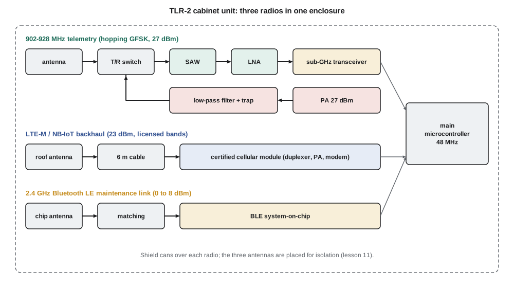
Amara starts from the requirements. The 902–928 MHz telemetry link stays, with the same frequency-hopping GFSK format at 50 kb/s, but its front end is redesigned: the cabinet unit gets a 27 dBm power amplifier, a surface acoustic wave (SAW) filter and an external low-noise amplifier so that cabinet-to-cabinet links can span 600 m with a large margin. A cellular modem using LTE-M or NB-IoT, the two low-power versions of LTE intended for machine connections, gives each cabinet a link to the traffic management system. A Bluetooth Low Energy (BLE) radio at 2.4 GHz in every pole and cabinet unit lets a technician's phone read status, logs and settings. A pole unit has two radios; a cabinet unit has all three.
| Radio | Band | Purpose | Key numbers |
|---|---|---|---|
| Telemetry | 902–928 MHz license-exempt | Poles to cabinet, cabinet to cabinet | 50 kb/s GFSK, 14 dBm pole, 27 dBm cabinet |
| Cellular backhaul | Licensed LTE bands, about 700 MHz to 2.2 GHz | Cabinet to traffic management system | 23 dBm class 3 module, a few kb/s average |
| Maintenance | 2.4 GHz license-exempt | Technician phone to any unit | BLE, 0 to 8 dBm, about 10 m |
Each radio raises different design problems. The telemetry radio is Cedarline's own design and the team controls everything in it, from the matching networks to the antenna. The cellular radio will be a certified module bought from a module maker, because designing and certifying an LTE modem is far beyond a small company; the team's work is the antenna, the cable, the layout around the module and the coexistence with the telemetry receiver a few centimeters away. The BLE radio is a system-on-chip with an integrated radio, and the work is the antenna and its matching on a crowded board.
The radio-frequency signal chain
Every radio receiver performs the same few tasks. It selects the wanted band and rejects others, amplifies a signal that may be as weak as a femtowatt, converts it to a frequency where it can be filtered and digitized, and recovers the information. Every transmitter does the reverse: it generates a modulated signal at a low frequency or in digital form, converts it to the carrier frequency, amplifies it to the required power and filters out everything the rules do not allow it to radiate. The way these tasks are arranged is the radio's architecture, and the choice of architecture fixes most of the performance before any circuit is designed.
Three quantities describe a receiver chain. Gain is the ratio of output to input power, usually in decibels. Noise figure (NF) measures how much the chain degrades the signal-to-noise ratio, and sets the weakest signal that can be received. Linearity, usually stated as the third-order intercept point (IIP3) referred to the input, or the 1 dB compression point, sets the strongest signals the chain can handle before it creates distortion products that bury the wanted signal. ELE-350 introduced all three; here they become the design variables.
Architectures
The superheterodyne receiver, invented about a century ago and still widely used, converts the incoming signal to a fixed intermediate frequency (IF) by mixing it with a local oscillator (LO). Because the IF is fixed, the channel filter and most of the gain can be built once and optimized, and the receiver is tuned by changing only the LO. The price is the image: a signal on the other side of the LO, one IF away from it, also mixes down to the IF and must be removed by a filter before the mixer. A high IF makes the image easy to filter but makes the channel filter harder; a low IF does the opposite. Many superheterodyne receivers use two conversions to get both benefits.
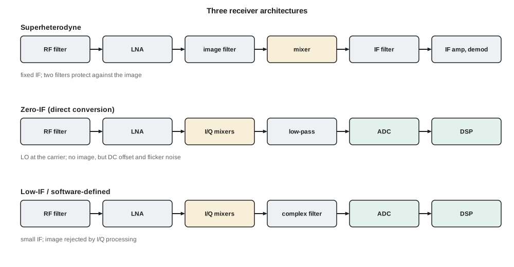
The zero-IF, or direct-conversion, receiver sets the LO at the carrier frequency and mixes directly to baseband in two paths, in-phase (I) and quadrature (Q), whose LOs differ by 90°. There is no image in the usual sense, because the image is the signal itself, and the channel filtering is done by simple low-pass filters that integrate well on a chip. Direct conversion has its own problems. The LO leaks to the antenna port and mixes with itself, producing a DC offset that can be larger than the wanted signal; second-order distortion converts strong amplitude-varying signals to baseband; and the flicker noise of transistors is largest at low frequencies, exactly where the signal now sits. Modern transceivers deal with these by calibration, high-pass filtering and careful layout, and direct conversion is now the usual choice for wideband cellular receivers.
The low-IF receiver, used in most sub-GHz and Bluetooth transceivers, mixes to an IF of a few hundred kilohertz to a few megahertz with I and Q paths and removes the image with a complex (polyphase) filter or in digital processing. It avoids the DC-offset and flicker-noise problems of zero-IF while keeping most of its integration benefits. The image is rejected by matching the I and Q paths rather than by a filter, so the rejection is limited to about 25 to 40 dB by gain and phase mismatch, as ELE-350 noted. The software-defined radio carries this idea further: the analog-to-digital converter sits as close to the antenna as power and cost allow, and filtering, demodulation and even the choice of standard are done in software.
The transceiver chip in TLR-1 is a low-IF design, and Amara keeps the same family for TLR-2 so that the software carries over. The cellular module uses direct conversion internally, and the BLE system-on-chip uses a low-IF receiver. The team does not design any of these architectures from scratch; it designs the circuits around them, and to do that well it must understand their weaknesses. Lesson 7 returns to the mixers and oscillators inside them.
Transmitter architectures
Transmitters have their own architectures. A direct-conversion transmitter generates I and Q baseband signals, converts them to analog and mixes them up to the carrier in one step; a polar transmitter separates amplitude and phase, driving a phase-modulated oscillator and modulating the amplitude through the power amplifier's supply. For a constant-envelope signal such as GFSK there is no amplitude to modulate at all: the synthesizer itself is modulated, and the power amplifier can run in saturation, which is why the TLR-1 transceiver can produce 14 dBm with good efficiency. The cellular module transmits signals whose amplitude varies, so its amplifier must be linear, a contrast that lesson 6 develops.
Cascade analysis of a receiver line-up
The first design decision for the TLR-2 telemetry receiver is what to put between the antenna and the transceiver chip. ELE-350 showed that the TLR-1 pole receiver, with a ceramic filter in front of a chip whose noise figure is 5 dB, has a system noise figure of 7 dB, while placing a low-noise amplifier first brings it near 1 dB. Lesson 7 of ELE-350 used the Friis formula for noise; the same cascade idea applies to linearity, with a twist that matters for TLR-2.
The noise formula says that the first stage dominates the noise figure if its gain is high. The linearity formula, with powers in milliwatts and gains as ratios, says the opposite for distortion: the later stages dominate, because they see the signal after it has been amplified. An LNA with 16 dB of gain in front of a transceiver whose IIP3 is −12 dBm lowers the input-referred IIP3 of the whole chain by about 16 dB. Gain improves sensitivity and degrades the ability to handle strong signals, and the designer has to strike a balance.
import math

# Cascade analysis of TLR-2 sub-GHz receiver line-ups at 915 MHz
def db(x): return 10 * math.log10(x)
def lin(d): return 10 ** (d / 10)

def cascade(stages):
    """stages: (name, gain dB, NF dB, IIP3 dBm). Returns gain, NF, IIP3 at the input."""
    g = 1.0; f = 1.0; inv_ip3 = 0.0
    for k, (name, gdb, nf, iip3) in enumerate(stages):
        f += (lin(nf) - 1) / g if k else lin(nf) - 1
        inv_ip3 += g / (lin(iip3) * 1e-3)        # refer each IIP3 to the input
        g *= lin(gdb)
    return db(g), db(f), db(1e3 / inv_ip3) if inv_ip3 else float('inf')

bw = 67.5e3          # noise bandwidth of the 50 kb/s GFSK channel, Hz
snr_req = 10.0       # SNR needed for the packet error target, dB
lineups = {
    'A: ceramic filter + chip (TLR-1 pole)': [('filter', -2.0, 2.0, 60), ('chip', 0, 5.0, -12)],
    'B: LNA + chip':                         [('LNA', 16, 1.0, 0), ('chip', 0, 5.0, -12)],
    'C: SAW + LNA + chip (TLR-2)':           [('SAW', -1.5, 1.5, 60), ('LNA', 16, 1.0, 0), ('chip', 0, 5.0, -12)],
}
for name, st in lineups.items():
    g, nf, iip3 = cascade(st)
    floor = -174 + db(bw) + nf          # noise floor in the channel, dBm
    sens = floor + snr_req
    sfdr = 2 / 3 * (iip3 - floor)       # spurious-free dynamic range, dB
    print(f"{name}")
print(f" gain {g:5.1f} dB NF {nf:4.2f} dB IIP3 {iip3:6.1f} dBm sensitivity {sens:6.1f} dBm SFDR {sfdr:4.1f} dB")A: ceramic filter + chip (TLR-1 pole) gain -2.0 dB NF 7.00 dB IIP3 -10.0 dBm sensitivity -108.7 dBm SFDR 72.5 dB B: LNA + chip gain 16.0 dB NF 1.18 dB IIP3 -28.0 dBm sensitivity -114.5 dBm SFDR 64.3 dB C: SAW + LNA + chip (TLR-2) gain 14.5 dB NF 2.68 dB IIP3 -26.5 dBm sensitivity -113.0 dBm SFDR 64.3 dB
The program compares three line-ups. Line-up A, the TLR-1 pole receiver, has the best linearity but the worst sensitivity, −108.7 dBm. Line-up B, an LNA straight into the chip, gives the best sensitivity, −114.5 dBm, but an input IIP3 of −28 dBm: two strong signals at −50 dBm each would create third-order products near the noise floor. Line-up C, Amara's choice for the cabinet, puts a SAW filter before the LNA. It gives up 1.5 dB of sensitivity, but the SAW removes strong cellular, paging and land-mobile signals outside 902–928 MHz before they reach the LNA, where they would otherwise compress it or create distortion. The spurious-free dynamic range, two-thirds of the distance between the noise floor and the IIP3, is the same for B and C, but C's applies only to signals inside the band, which is where it matters.
Worked problem
Sensitivity of line-up C
Line-up C has a cascade noise figure of 2.68 dB, a noise bandwidth of 67.5 kHz and needs a 10 dB SNR. Find its sensitivity.
Show solution
- \[P_{min} = -174 + 10\log_{10}(67\,500) + \mathrm{NF} + \mathrm{SNR}\]
- \[P_{min} = -174 + 48.3 + 2.68 + 10 = -113.0\ \text{dBm}\]
- Compared with TLR-1's −108.7 dBm this is 4.3 dB better, which adds about 4 dB to every link margin.
Answer: About −113 dBm.
Worked problem
Distortion from two strong signals
Two signals at 909 and 910 MHz arrive at the cabinet receiver at −40 dBm each. Line-up C has an input IIP3 of −26.5 dBm. Where do the third-order products fall and how strong are they?
Show solution
- Third-order products fall at 2f₁ − f₂ = 908 MHz and 2f₂ − f₁ = 911 MHz, inside the band and therefore not removed by the SAW.
- \[P_{IM3} = 3P_{in} - 2\,\mathrm{IIP3} = 3(-40) - 2(-26.5) = -67\ \text{dBm}\]
- That is 46 dB above the −113 dBm sensitivity. A hopping channel at 908 or 911 MHz would be blocked while both signals are present, which is one reason the link uses retries and frequency hopping.
Answer: At 908 and 911 MHz, about −67 dBm referred to the input.
Dynamic range and blocking
Sensitivity and IIP3 are not the only limits. A receiver must also tolerate a single strong signal close to the wanted one, called a blocker, without losing sensitivity. A blocker can compress the LNA, reducing its gain; it can mix with the LO's phase noise and land in the channel, as lesson 7 shows; and it can be strong enough to overload the analog-to-digital converter. Data sheets state blocking performance as the level of an interferer at given frequency offsets that causes a specified loss of sensitivity, and the TLR-2 specification includes a blocking requirement taken from the worst signals Leo measured at three busy intersections: a cellular uplink at 849 MHz from a phone in a car stopped beside the cabinet, and land-mobile radio transmitters near 460 MHz used by the city's own trucks.
Leo's survey also found a paging transmitter near 930 MHz, only 2 MHz above the band edge, at about −35 dBm at the cabinet antenna. No affordable SAW filter can reject a signal that close by more than a few decibels, so the transceiver's own selectivity must handle it. Amara adds the measured levels to the requirement list; they will drive the filter choice in lesson 4 and the coexistence work in lesson 11.
Planning the TLR-2 project
Amara divides the work by risk. The telemetry front end is mostly Cedarline's own circuitry, so its matching networks, LNA, power amplifier and harmonic filter are designed and measured first. The cellular backhaul is lower risk in the circuits, because the module is certified, but higher risk in the system: antenna placement, cable loss, coverage at each cabinet and carrier approval. The BLE link is the simplest, but its tiny antenna must work in a metal pole housing. Daniel insists that every radio-frequency design decision be backed by a measurement on a test fixture before the full board is laid out, a rule that lesson 2 makes possible by teaching how such measurements are made.
Common mistakes
MistakePutting an LNA first in every receiver because it gives the lowest noise figure.
InsteadGain before the strongest-signal stage lowers the chain's IIP3; a filter in front often gives a better overall result.
MistakeAssuming a zero-IF receiver has no image problem at all.
InsteadIt has no separate image band, but I/Q mismatch, DC offset and flicker noise become the limits.
MistakeAdding noise figures in decibels along a chain.
InsteadNoise factors combine as ratios through the Friis formula; each stage's contribution is divided by the gain before it.
MistakeJudging a receiver by sensitivity alone.
InsteadBlocking, intermodulation and selectivity often decide whether a radio works in a busy urban spectrum.
Summary and key terms
- A receiver selects, amplifies, converts and demodulates; a transmitter generates, converts, amplifies and filters. The arrangement is the architecture.
- Superheterodyne receivers use a fixed IF and must reject the image; zero-IF receivers avoid the image but suffer DC offset and flicker noise; low-IF receivers reject the image with I/Q processing.
- Noise figure is dominated by the first stages, linearity by the last; gain improves one and degrades the other.
- Sensitivity is −174 dBm/Hz + 10 log B + NF + required SNR.
- Spurious-free dynamic range is two-thirds of the distance from the noise floor to the IIP3.
- TLR-2 combines a redesigned 902–928 MHz telemetry radio, an LTE-M or NB-IoT cellular module and a BLE maintenance radio.
- Architecture
- The arrangement of filters, amplifiers, mixers and converters in a radio.
- Intermediate frequency (IF)
- The fixed frequency to which a superheterodyne receiver converts the signal.
- Image
- A signal one IF on the other side of the LO that also converts to the IF.
- Zero-IF receiver
- A receiver that converts directly to baseband with I and Q mixers.
- Low-IF receiver
- A receiver that converts to a small IF and rejects the image with I/Q processing.
- Input third-order intercept (IIP3)
- The extrapolated input power at which third-order products would equal the fundamental.
- Blocker
- A strong unwanted signal near the wanted frequency that can reduce sensitivity.
- Spurious-free dynamic range
- The range of input power over which signals are above the noise and their distortion is below it.
Practice problems
Work each problem on paper first, then reveal the answer to check.
A receiver has NF 3 dB, noise bandwidth 200 kHz and needs SNR 8 dB. What is its sensitivity?
Show answer
−174 + 53.0 + 3 + 8 = −110 dBm.
A filter with 2 dB loss is placed in front of an LNA with NF 1 dB. What is the combined noise figure, ignoring later stages?
Show answer
The filter's noise figure equals its loss, 2 dB; the combination is about 3 dB.
An LNA with 20 dB gain and IIP3 0 dBm drives a mixer with IIP3 +5 dBm. Find the cascade IIP3.
Show answer
1/IIP3 = 1/1 + 100/3.16 = 32.6 per milliwatt, so IIP3 ≈ 0.031 mW ≈ −15.1 dBm.
An FM broadcast receiver uses a 10.7 MHz IF with high-side LO. Where is the image for a station at 100.1 MHz?
Show answer
LO 110.8 MHz; image 121.5 MHz.
Why does a direct-conversion receiver suffer from flicker noise?
Show answer
Its signal is converted to near zero frequency, where transistor flicker noise is largest.
Two signals at 912 and 914 MHz enter a receiver. Where are their third-order products?
Show answer
910 and 916 MHz.
Lesson quiz · 5 questions
Score 60% or more to complete this lesson.
Create a free account to save your progress, take quizzes and earn a certificate.