Layout, parasitics and matching

The schematic of the CX-1 preamplifier says which transistors connect to which; the layout says where they are, how big they are, how the wires run and what lies next to them. Two layouts of the same schematic can differ in offset by a factor of five, in bandwidth by a factor of two and in the amount of clock noise they pick up from the digital half by a factor of a hundred. This lesson covers the craft of layout: stick diagrams and cell planning, the parasitic resistance and capacitance of wiring and how to estimate their delay, and the matching techniques that let the CX-1 analog blocks meet their specifications despite the random variation that lesson 2 introduced.

From schematic to geometry

A layout is built from rectangles and polygons on each layer. A transistor is the intersection of a poly line with an active area; contacts connect active and poly to metal 1; vias connect each metal layer to the next. Designers plan layouts with stick diagrams, quick sketches that show each layer as a colored line, transistors where poly crosses active, and contacts as crosses, without dimensions. A stick diagram of a NAND2, for example, shows two vertical poly lines crossing a horizontal n-active strip at the bottom and a p-active strip at the top, with the supply rails running along the top and bottom edges. The diagram fixes the topology and the order of devices, and therefore which diffusions can be shared between neighboring transistors.

Diffusion sharing is the first layout optimization. Two transistors in series, or two in parallel with a common terminal, can share one diffusion region rather than each having its own, which saves area and, more importantly for speed, junction capacitance. Standard cells are drawn so that their transistors form unbroken strips of n and p active area wherever the logic allows, a problem that for complex gates becomes finding a path through the gate's graph that visits every transistor once. All cells in a library share the same height, with power rails at the top and bottom, so that the place-and-route tool can abut them in rows.

Wide transistors are drawn as several fingers in parallel, each a poly line across the same active area, with alternating source and drain diffusions between them. A 40 µm transistor drawn as eight fingers of 5 µm is compact and nearly square, its gate resistance is divided by eight, and the drains shared between fingers have half the junction area of a single wide device. The CX-1 preamplifier's input transistors, which lesson 9 sizes at about 79 µm wide and 1 µm long, will be drawn as sixteen fingers of about 5 µm.

Wiring parasitics

Every wire is a distributed resistor and capacitor. Its resistance follows from the metal's sheet resistance and the number of squares along it. Its capacitance has three parts: the parallel-plate capacitance to the substrate or the layer below, the fringing capacitance from its edges, and the coupling capacitance to its neighbors on the same layer. In a 180 nm process a minimum-width metal line has about 0.15 to 0.25 fF per micrometer in total, with coupling to neighbors often the largest part. Coupling matters twice: it adds to the wire's load, and it injects a fraction of every neighboring signal's swing as crosstalk.

For a long wire, the Elmore delay gives a simple and surprisingly good estimate. The wire is modeled as a ladder of resistors and capacitors; the Elmore delay to the far end is the sum, over every capacitor, of that capacitor times the total resistance between it and the driver. For a uniform distributed line of total resistance R and capacitance C, driven through a resistance R_d into a load C_L, the sum becomes a short formula.

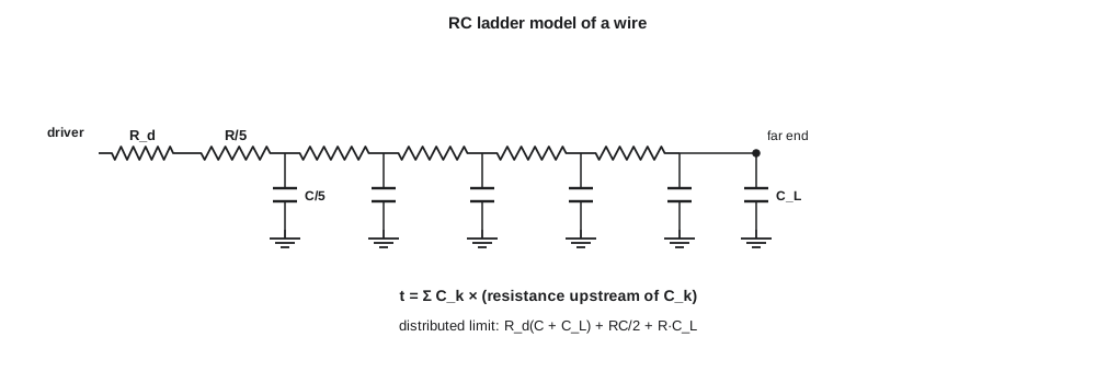
Amara uses it for the 2 mm clock route from the CX-1 clock buffer to the counter block.

import random
# 1. Elmore delay of a 2 mm metal-2 route from the clock buffer to the counter block
r_sq, w_um = 0.08, 0.28            # ohms per square, wire width um
c_per_um = 0.20e-15                # F per um including fringe and coupling
length = 2000.0                    # um
r_drv, c_load = 400.0, 50e-15      # driver resistance, receiver load
R = r_sq * length / w_um
Cw = c_per_um * length
def elmore(nseg, r_drv, R, Cw, cl):
    r, c = R / nseg, Cw / nseg
    t = 0.0
    for k in range(1, nseg + 1):
        t += (r_drv + k * r) * c         # each segment cap sees the resistance upstream
    return t + (r_drv + R) * cl
print(f"wire R = {R:.0f} ohm, C = {Cw * 1e15:.0f} fF")
for n in (1, 4, 20, 200):
    print(f"  {n:>3} segments: Elmore delay {elmore(n, r_drv, R, Cw, c_load) * 1e12:.1f} ps")
print(f"  distributed limit check: RdC + RdCl + RC/2 + RCl = {(r_drv * (Cw + c_load) + R * Cw / 2 + R * c_load) * 1e12:.1f} ps")

# 2. Linear oxide gradient across a pair of input transistors: why common centroid works
grad = 0.20e-3        # threshold gradient, V per um across the die region
pitch = 6.0           # um between unit fingers
def offset(pattern):
    a = [i * pitch for i, s in enumerate(pattern) if s == "A"]
    b = [i * pitch for i, s in enumerate(pattern) if s == "B"]
    return grad * (sum(a) / len(a) - sum(b) / len(b))
for pat in ("AABB", "ABAB", "ABBA", "AABBAABB", "ABBAABBA"):
    print(f"  pattern {pat:<9} systematic offset {offset(pat) * 1e3:+.2f} mV")

# 3. Random mismatch does not care about the pattern (Pelgrom, A_VT = 4 mV um)
random.seed(7)
avt, W, L = 4.0e-3, 20.0, 1.0
sigma = avt / (W * L) ** 0.5
samples = [random.gauss(0, sigma) for _ in range(2000)]
s = (sum(x * x for x in samples) / len(samples)) ** 0.5
print(f"random offset sigma for W/L = {W:.0f}/{L:.0f}: predicted {sigma * 1e3:.2f} mV, simulated {s * 1e3:.2f} mV")

wire R = 571 ohm, C = 400 fF
    1 segments: Elmore delay 437.1 ps
    4 segments: Elmore delay 351.4 ps
   20 segments: Elmore delay 328.6 ps
  200 segments: Elmore delay 323.4 ps
  distributed limit check: RdC + RdCl + RC/2 + RCl = 322.9 ps
  pattern AABB      systematic offset -2.40 mV
  pattern ABAB      systematic offset -1.20 mV
  pattern ABBA      systematic offset +0.00 mV
  pattern AABBAABB  systematic offset -2.40 mV
  pattern ABBAABBA  systematic offset +0.00 mV
random offset sigma for W/L = 20/1: predicted 0.89 mV, simulated 0.91 mV

The 2 mm metal-2 route has 571 Ω of resistance and 400 fF of capacitance. A single lumped segment overestimates the delay at 437 ps; twenty segments give 329 ps, within 2 % of the distributed limit of 323 ps. The wire's own RC/2 term, about 114 ps, is a third of the total, and it grows with the square of length, which is why long wires on fast chips are broken up with repeaters. At 20 MHz the delay is harmless, but the route's 400 fF switching every cycle costs about 26 µW at 1.8 V, a noticeable share of the budget of lesson 6, which is why Priya asks for the counter block to be placed next to the clock buffer.

Substrate and supply noise

The digital half of CX-1 is the analog half's worst enemy. Every clock edge draws a burst of current from the supply, and the supply wires' resistance and the package's bond-wire inductance turn that current into voltage spikes on the digital supply and ground. The same edges inject charge into the shared substrate through junction capacitances, and the substrate carries it to every analog transistor's body. The CX-1 microphone preamplifier, which amplifies millivolt signals, would hear the 20 MHz clock as noise if nothing were done.

The defenses are layout disciplines. The analog and digital blocks have separate supply and ground pins and separate on-chip supply networks, joined only at the package or the board. Digital and analog blocks sit at opposite ends of the die, with the bias and reference circuits, which are the most sensitive, furthest from the counters. Guard rings of substrate contacts tied to a quiet ground surround the analog blocks and collect injected charge before it reaches them; n-well guard rings tied to the supply add a second barrier. Sensitive analog nodes are routed on upper metal layers, well away from clock lines, and shielded where they must run near digital signals. On-chip decoupling capacitance on each supply, built from MOS capacitors in otherwise empty space, supplies the fast current bursts locally. And the analog circuits themselves are designed to be differential where possible, so that noise common to both sides is rejected.

Matching

Analog precision on a chip comes from matching. A differential pair has offset because its two transistors are not identical; a current mirror copies its reference with an error because its devices differ; a data converter's linearity depends on how well its capacitors match. Mismatch has two components, which call for different remedies.

Systematic mismatch comes from causes that vary smoothly across the die, such as gradients in oxide thickness, doping, temperature or mechanical stress, and from layout asymmetries, such as one device having a wire run beside it that the other does not. Systematic mismatch can be canceled by placement. Random mismatch comes from the atomic-scale randomness of each device, the number and position of dopant atoms under its gate and the roughness of its edges. It cannot be canceled, only reduced by making devices larger.

Common-centroid layout

If a parameter varies linearly across the die, two devices whose centers of gravity coincide see the same average value, and the gradient cancels. This is the principle of common-centroid layout. Each device is split into an even number of unit fingers, and the units are arranged so that the centroid of device A's units falls on the centroid of device B's. In one dimension the pattern ABBA is common-centroid; AABB is not. In two dimensions a cross-coupled quad, A and B on one diagonal each, cancels gradients in both directions.

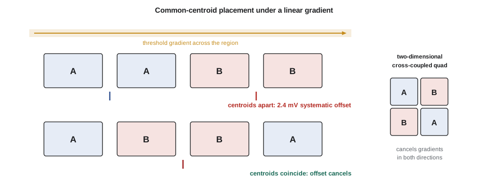
The script places four unit fingers of a differential pair at a 6 µm pitch under a threshold gradient of 0.2 mV per micrometer. The simple AABB arrangement gives a systematic offset of 2.4 mV, larger than the random offset budget for the whole preamplifier. Interdigitating as ABAB halves it but does not remove it, because the centroids still differ by one pitch. ABBA cancels it exactly, and so does the longer ABBAABBA. Common-centroid placement removes linear gradients only; quadratic terms remain, which is why the most precise layouts use more units arranged in more elaborate patterns.

Several other rules complete good matching practice. Matched devices have the same orientation, because the crystal and the implant tilt make transistor properties differ with direction. They have the same surroundings: dummy devices, unconnected fingers at the ends of each array, ensure that every active finger sees a neighbor on both sides, so that edge effects in etching and stress are the same. They are placed close together and away from the edges of wells, where doping changes. They carry the same current density and see the same temperature, which means they are kept away from the power devices and placed on a line of thermal symmetry if there is one. And they are connected with wiring that is itself symmetric, so that neither device sees more series resistance or coupling than its partner.

Pelgrom's law

Random mismatch follows a remarkably consistent law, published by Marcel Pelgrom and colleagues in 1989. For two identically drawn, closely spaced transistors, the standard deviation of the difference in threshold voltage, and of the fractional difference in current factor, is inversely proportional to the square root of the gate area.

The coefficient A_VT is roughly proportional to gate oxide thickness and is about 3 to 5 mV·µm for a 180 nm process; the illustrative CX-1 value is 4 mV·µm for NMOS and 5 mV·µm for PMOS. A pair of 20 µm by 1 µm devices therefore has a threshold mismatch with a standard deviation of 4/√20 ≈ 0.9 mV; the script's 2 000 random samples confirm it. To halve the mismatch the area must quadruple. This square-root law is the fundamental cost of analog precision in CMOS: accuracy is paid for in area, and with area comes capacitance, which costs speed or power.

Parasitic extraction and the post-layout loop

Once a block's layout is drawn and passes DRC and LVS, an extraction tool computes the resistance and capacitance of every net, including coupling between nets, and writes a netlist that includes them. Post-layout simulation of that netlist is where a designer learns whether the layout has cost too much. For analog blocks the common surprises are extra capacitance on high-impedance nodes, which lowers a pole frequency and erodes phase margin; resistance in the source connections of wide devices, which degenerates them and lowers their transconductance; and coupling from a digital line into a sensitive node. Priya's rule for CX-1 is that every analog block is simulated after extraction across corners, and its phase margin and offset must still meet specification with margin before the block is released.