Designing, simulating and verifying circuits

The previous lessons analyzed circuits that were given. Engineering runs the other way: you start from a requirement and must produce a circuit that meets it in every unit built, over its whole range of temperature and supply voltage, for years, and safely. This final lesson brings the course together as a design process. It covers turning requirements into a circuit, choosing standard component values, verifying the design by worst-case and Monte Carlo analysis, building and measuring prototypes, the physical realities of printed circuit boards, and the safety standards and reviews that stand between a design and a product.

The design process

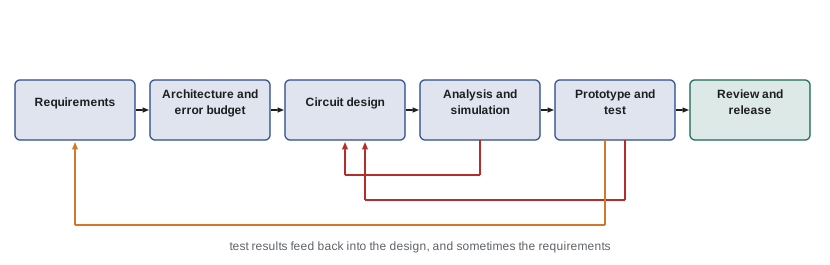
Most circuit design follows the same loop, whether the result is a sensor interface or a power supply:

1. Requirements: what the circuit must do, quantitatively. Input and output ranges, accuracy, power consumption, supply voltages, operating temperature, size, cost, and the standards it must meet.

2. Architecture: the blocks and how they connect, for example sensor, bridge, in-amp, ADC (Lesson 9), with an error budget allocating the allowed error among them.

3. Circuit design: choose topologies and calculate component values with the methods of this course.

4. Verification by analysis and simulation: check nominal performance, then tolerances, temperature and worst cases (Lesson 5).

5. Prototype and test: build, measure, compare with predictions, and find what the models missed.

6. Review, documentation and release: independent design review, a bill of materials, test procedures and the evidence needed for certification.

The loop repeats: test results feed back into the design, and requirements themselves are often revised when their cost becomes clear.

From requirement to values

Calculated component values rarely match standard values. The designer picks from the E-series (Lesson 3), often by searching combinations for the best fit, while also respecting other constraints such as current consumption, loading and noise.

import itertools
import numpy as np

E24 = [1.0, 1.1, 1.2, 1.3, 1.5, 1.6, 1.8, 2.0, 2.2, 2.4, 2.7, 3.0,
       3.3, 3.6, 3.9, 4.3, 4.7, 5.1, 5.6, 6.2, 6.8, 7.5, 8.2, 9.1]
values = [m * 10**d for d in range(3, 6) for m in E24]   # 1 kOhm to 910 kOhm

target = 3.3 / 5.0          # divide 5 V down to 3.3 V
best = sorted(((abs(r2 / (r1 + r2) - target), r1, r2) for r1, r2 in itertools.product(values, values)
               if 10e3 <= r1 + r2 <= 200e3))[:3]
for err, r1, r2 in best:
    vout = 5.0 * r2 / (r1 + r2)
    print(f"R1 = {r1 / 1e3:g} k, R2 = {r2 / 1e3:g} k -> {vout:.4f} V (error {err / target:.3%}), "
          f"current {5.0 / (r1 + r2) * 1e6:.0f} uA")

R1 = 4.7 k, R2 = 9.1 k -> 3.2971 V (error 0.088%), current 362 uA
R1 = 47 k, R2 = 91 k -> 3.2971 V (error 0.088%), current 36 uA
R1 = 6.2 k, R2 = 12 k -> 3.2967 V (error 0.100%), current 275 uA

Two pairs give identical ratios, 4.7 k with 9.1 k and 47 k with 91 k, both within 0.09% of the target, but they differ tenfold in current. The choice depends on the rest of the design: the lower-value pair wastes 362 µA but tolerates more loading; the higher-value pair saves power, which matters in battery-powered sensors, but must drive only a high-impedance input (Lesson 3). Searching costs nothing, and the computer is never tempted to stop at the first acceptable answer.

Worst-case and Monte Carlo analysis

Worst-case analysis sets every component to the limit that pushes the output furthest, guaranteeing that every unit meets the result. For circuits with many components it becomes very pessimistic, because it assumes all errors line up at once. Monte Carlo analysis instead simulates thousands of virtual units, each with component values drawn at random within their tolerances, and reports the distribution of the output, giving the expected yield: the fraction of units that will meet a specification.

import numpy as np

rng = np.random.default_rng(202)
N = 100_000
Vs = 12.0

def divider(tol, dist):
    if dist == "uniform":
        R1 = 10e3 * (1 + rng.uniform(-tol, tol, N))
        R2 = 10e3 * (1 + rng.uniform(-tol, tol, N))
    else:  # normal, with the tolerance as 3 standard deviations
        R1 = 10e3 * (1 + rng.normal(0, tol / 3, N))
        R2 = 10e3 * (1 + rng.normal(0, tol / 3, N))
    return Vs * R2 / (R1 + R2)

for tol in [0.05, 0.01]:
    for dist in ["uniform", "normal"]:
        v = divider(tol, dist)
        inside = np.mean(np.abs(v - 6.0) <= 0.06)
        print(f"+/-{tol:.0%} {dist:>7}: mean {v.mean():.4f} V, sd {v.std() * 1e3:5.1f} mV, "
              f"range {v.min():.3f}-{v.max():.3f} V, within 6.00 +/- 0.06 V: {inside:.1%}")

+/-5% uniform: mean 5.9999 V, sd 122.8 mV, range 5.701-6.298 V, within 6.00 +/- 0.06 V: 35.7%
+/-5%  normal: mean 5.9999 V, sd  70.7 mV, range 5.669-6.305 V, within 6.00 +/- 0.06 V: 60.3%
+/-1% uniform: mean 6.0000 V, sd  24.5 mV, range 5.940-6.060 V, within 6.00 +/- 0.06 V: 100.0%
+/-1%  normal: mean 6.0000 V, sd  14.1 mV, range 5.937-6.058 V, within 6.00 +/- 0.06 V: 100.0%

Several lessons are visible. With ±5% resistors, only 36% to 60% of dividers fall within ±1% of 6 V, depending on how values are distributed within tolerance; with ±1% resistors, essentially all do. The distribution assumption matters: manufacturers do not promise a shape, and parts are sometimes selected from a batch so that the tightest ones are sold as a better grade, leaving a distribution with a hole in the middle. And the normal model with the tolerance at three standard deviations even produces a few values slightly beyond the worst-case range, a reminder that statistical models of tolerance are approximations. For guarantees, use worst case; for cost and yield estimates, use Monte Carlo with realistic distributions, ideally measured.

Temperature and derating

A design must work across its specified temperature range, typically 0 °C to 70 °C for commercial equipment, −40 °C to 85 °C for industrial equipment and wider for automotive and aerospace. Every temperature-dependent parameter, resistor TCR, op amp offset drift, reference voltage drift, battery capacity, capacitor life (Lesson 10), must be checked at the extremes. Derating, operating components well below their maximum ratings of power, voltage, current and temperature, is the most effective way to improve reliability. Common rules include running resistors at no more than 50% of their derated power, capacitors at no more than 50% to 80% of their voltage rating, and semiconductors well below their maximum junction temperature.

Printed circuit boards are circuits too

On a printed circuit board (PCB), every copper trace is a resistor, and at high currents its resistance matters. The resistance of a trace is \(R = \rho L/(wt)\), where for standard "1 ounce" copper the thickness \(t\) is about 35 µm, giving a sheet resistance of about 0.5 mΩ per square: a trace 1 mm wide and 10 mm long (10 squares) has about 5 mΩ.

Ground is not a single point either. Shared ground paths carry the currents of several circuits, and the small voltage drops along them appear as errors in sensitive measurements. Good layout keeps high-current return paths away from precision circuits, uses ground planes, and connects sensitive references at a single point (star grounding), applying KVL around every loop that includes a shared conductor.

Building and measuring prototypes

A prototype tests both the design and the models used to design it. Good laboratory practice includes:

• Use a bench supply with its current limit set just above the expected current, so that a wiring mistake or a faulty part limits current instead of destroying parts.
• Power up in stages: check supply rails with no load, then add blocks one at a time, measuring current at each step.
• Measure, then compare with predictions: node voltages, currents and temperatures. A difference is information; find out which model was wrong.
• Account for instruments: meter loading and burden (Lesson 3), probe ground connections, and the uncertainty of each instrument.
• Record everything: settings, measurements, changes and observations, so that results can be traced and repeated.

Safety, standards and reviews

Electrical products must be safe in normal use and under foreseeable faults. Safety standards set requirements for insulation, spacing between conductors (creepage and clearance), protection against overheating and fire, and protective earthing, and certified test laboratories verify compliance.

In the US, electrical products are commonly certified to UL standards (for example UL 62368-1 for information and communication technology equipment) by a Nationally Recognized Testing Laboratory, as required by OSHA for workplace equipment and by local electrical codes. Professional engineers who take legal responsibility for designs are licensed by state boards.

Independent design review, in which experienced engineers who did not create the design examine it, catches errors that the designer cannot see: a missed worst case, a component used beyond its rating, an untested failure mode. Checklists, peer review of calculations and simulation files, and traceability from each requirement to the analysis or test that verifies it are standard practice in every serious engineering organization.

Where the course leads

This course has covered the analysis of DC circuits: the elements, Kirchhoff's laws, nodal and mesh analysis, matrix methods, theorems, dependent sources and two-ports, op amps and their applications, energy storage, power and design. Circuit Analysis II (ELE-203) adds time and frequency: transients in RC and RL circuits, phasors and impedance, AC power, three-phase systems and filters. Electronics I (ELE-240) replaces the dependent-source models with real diodes and transistors, and later courses build on both for power systems, machines, power electronics, signals, communications and control.