
CON-350 · Lesson 3 of 12 · 25 min
Qualitative and quantitative risk analysis
Once risks are identified, the team must decide which matter most. A register for a medium-sized building can easily hold sixty or eighty risks, and nobody can manage them all with equal attention. Risk analysis sorts them: qualitative analysis ranks risks quickly using scales, and quantitative analysis estimates their combined effect on cost and schedule in dollars and days. Both have a place. Qualitative scoring is fast, cheap and good enough for most risks; quantitative analysis takes more effort but answers the questions owners and lenders ask, such as how much contingency is needed and how likely the project is to finish on time.
Probability and impact scales
Qualitative analysis assigns each risk a probability score and an impact score, usually on scales of 1 to 5. The scales must be defined in words and, where possible, numbers, so that different people score the same risk the same way. Scales without definitions produce scores that mean different things to different people.
| Score | Probability | Cost impact (Kingfisher Wharf) | Schedule impact | Safety impact |
|---|---|---|---|---|
| 1 Rare / Minor | Under 5 % | Under $50,000 | Under 1 week | First aid |
| 2 Unlikely / Moderate | 5 to 20 % | $50,000 to $250,000 | 1 to 2 weeks | Medical aid |
| 3 Possible / Significant | 20 to 50 % | $250,000 to $750,000 | 2 to 6 weeks | Lost time injury |
| 4 Likely / Major | 50 to 80 % | $750,000 to $2 million | 6 to 12 weeks | Serious injury |
| 5 Almost certain / Severe | Over 80 % | Over $2 million | Over 12 weeks or misses opening | Death or multiple serious injuries |
Impact scales should be tied to the size of the project and the organization's tolerance. A $250,000 impact is significant on a $48 million building but trivial on a $2 billion transit line. Where a risk affects several objectives, the usual rule is to score the worst one, so a risk with minor cost but serious safety consequences scores high. Safety risks are often handled separately with their own hazard assessment process (HSE-103), and a fatality is never traded off against dollars.
The probability-impact matrix
Multiplying probability by impact gives a score from 1 to 25, and plotting risks on a 5 × 5 grid, the probability-impact matrix or heat map, shows the pattern at a glance. Cells are shaded into bands: high (red) risks need immediate action and senior attention, medium (amber) risks need planned responses, and low (green) risks are monitored.
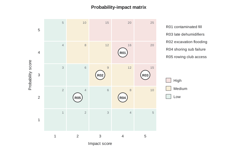
The matrix has known weaknesses. Multiplying ordinal scores is mathematically dubious, because a 4 is not twice a 2. Very different risks can share a score: a near-certain small loss and a rare catastrophe can both score 5. Scores also hide the size of the loss within a band. Many organizations therefore weight impact more heavily than probability, mark any risk with an impact of 5 as high regardless of probability, or move to quantitative methods for the top risks. The matrix remains a useful sorting tool as long as everyone remembers what it can and cannot tell them.
Expected monetary value
The simplest quantitative measure is expected monetary value (EMV): the probability of the risk multiplied by its cost if it occurs. A 30 % chance of a $600,000 loss has an EMV of $180,000. Summing the EMVs of independent risks gives a first estimate of how much money the project should expect to spend on them, which is a starting point for contingency.
Worked problem
Expected monetary value for four risks
Tallgrass Builders estimates four contractor-carried risks: excavation flooding (30 %, $400,000), late dehumidifiers causing acceleration (35 %, $520,000), shoring subcontractor failure (10 %, $900,000) and tile rework in the pool (20 %, $250,000). What is the total EMV?
Show solution
- Flooding: 0.30 × 400,000 = $120,000.
- Dehumidifiers: 0.35 × 520,000 = $182,000.
- Shoring failure: 0.10 × 900,000 = $90,000.
- Tile rework: 0.20 × 250,000 = $50,000.
- Total: 120,000 + 182,000 + 90,000 + 50,000 = $442,000.
Answer: Total EMV is $442,000. The project should expect to spend about this much on these risks, but in any single outcome it will spend either nothing or the full cost for each risk, so the actual figure could be much higher or lower.
EMV is easy to explain but has a trap. The expected value is an average over many hypothetical repetitions of the project, and each project happens only once. If the shoring subcontractor fails, the cost is $900,000, not $90,000. A contingency set at the total EMV will therefore be exceeded quite often. To know how often, the team needs the whole distribution of outcomes, which is what Monte Carlo simulation provides.
Three-point estimates and distributions
Quantitative analysis replaces single numbers with ranges. For each uncertain cost item or risk, the estimator gives three values: an optimistic minimum, a most likely value and a pessimistic maximum. These define a probability distribution. The two common choices are the triangular distribution, which uses the three points directly, and the PERT (beta-PERT) distribution, which gives more weight to the most likely value and less to the tails.
| Distribution | Mean | Character |
|---|---|---|
| Triangular | (a + m + b) ÷ 3 | Simple; tails relatively heavy |
| PERT | (a + 4m + b) ÷ 6 | Smoother; concentrates near the most likely value |
| Uniform | (a + b) ÷ 2 | No most likely value; used when nothing is known within the range |
| Discrete (risk event) | p × impact | Either happens or not; impact may itself be a range |
Two kinds of uncertainty go into the model. Estimating uncertainty covers the normal spread in quantities and rates: concrete may cost a little more or less than estimated. Risk events are discrete: they either happen or they do not. A good model includes both, with each risk event modeled as a probability of occurrence and an impact range if it occurs.
Monte Carlo simulation
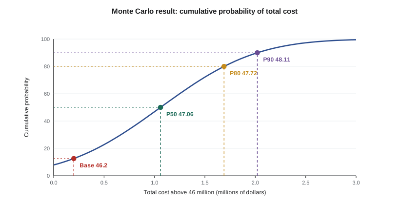
Monte Carlo simulation combines the distributions by sampling. The computer draws a random value for every uncertain item and decides at random whether each risk event occurs, adds everything up to get one possible project cost, and repeats the process thousands of times. The results form a distribution of total cost, usually shown as an S-curve of cumulative probability. From the S-curve the team reads percentiles: the P50 is the cost with a 50 % chance of not being exceeded, the P80 has an 80 % chance, and so on.
# Monte Carlo cost risk analysis for Kingfisher Wharf (illustrative, seeded)
import numpy as np
rng = np.random.default_rng(350)
N = 20_000
base = 46_200_000          # point estimate before contingency, $

# estimating uncertainty: (min, most likely, max) as fractions of three cost groups
groups = {"structure": (0.97, 1.00, 1.08, 15_400_000),
          "mechanical/electrical": (0.96, 1.00, 1.12, 13_900_000),
          "other trades": (0.98, 1.00, 1.06, 16_900_000)}
def pert(a, m, b, size):
    alpha = 1 + 4 * (m - a) / (b - a); beta = 1 + 4 * (b - m) / (b - a)
    return a + rng.beta(alpha, beta, size) * (b - a)
total = np.zeros(N)
for a, m, b, value in groups.values():
    total += pert(a, m, b, N) * value

# risk events: probability, (min, most likely, max) impact in $
events = [(0.30, (200_000, 400_000, 700_000)),    # excavation flooding
          (0.35, (300_000, 520_000, 900_000)),    # late dehumidifiers, acceleration
          (0.10, (600_000, 900_000, 1_500_000)),  # shoring subcontractor failure
          (0.20, (120_000, 250_000, 450_000))]    # pool tile rework
for p, (a, m, b) in events:
    occurs = rng.random(N) < p
    total += occurs * rng.triangular(a, m, b, N)

for q in (10, 50, 80, 90):
    print(f"P{q}: ${np.percentile(total, q):,.0f}  (contingency over base {np.percentile(total, q) - base:,.0f})")
print(f"Mean: ${total.mean():,.0f}")
print(f"Chance the base estimate is enough: {np.mean(total <= base):.1%}")P10: $46,211,223 (contingency over base 11,223) P50: $47,063,630 (contingency over base 863,630) P80: $47,717,848 (contingency over base 1,517,848) P90: $48,105,209 (contingency over base 1,905,209) Mean: $47,117,817 Chance the base estimate is enough: 9.6%
The output shows something every estimator should absorb: the point estimate, built from most likely values, has only a small chance of being enough. Most likely values are usually closer to the optimistic end of each range, because things can go much more wrong than right, so the sum of most likely values sits low on the S-curve. The gap between the base and the P80 is a defensible contingency for an owner who wants an 80 % chance of staying in budget. Lesson 4 discusses how organizations choose that confidence level.
Schedule risk analysis
The same method applies to time. Each activity in the schedule gets a duration range, risk events are attached to the activities they would affect, and the simulation runs the critical path calculation thousands of times. Schedule risk analysis reveals two things a deterministic schedule hides. First, the finish date is uncertain, and the deterministic date often has a low probability. Second, merge bias: where several paths converge, the chance that all of them finish on time is lower than the chance for any one, so converging paths push the probable finish later.
# Merge bias: two parallel paths feeding one milestone (illustrative, seeded)
import numpy as np
rng = np.random.default_rng(7)
N = 50_000
# pool hall enclosure path and parking structure path, weeks (min, most likely, max)
pool = rng.triangular(20, 24, 34, N)
parking = rng.triangular(21, 24, 32, N)
finish = np.maximum(pool, parking)
for name, d in (("pool path", pool), ("parking path", parking), ("milestone", finish)):
print(f"{name:<13} P(<= 24 weeks) = {np.mean(d <= 24):.1%} P80 = {np.percentile(d, 80):.1f} weeks")pool path P(<= 24 weeks) = 28.5% P80 = 28.7 weeks parking path P(<= 24 weeks) = 27.4% P80 = 27.8 weeks milestone P(<= 24 weeks) = 7.8% P80 = 29.6 weeks
Each path on its own has a modest chance of meeting 24 weeks, but the milestone, which needs both, has a much lower chance. That is merge bias, and it explains why projects with many parallel trades finishing at the same time so often run late. Integrated cost and schedule risk models go a step further by linking time to cost, so that a delay also adds the time-related costs of site overhead, equipment and escalation. CON-210 covers scheduling, and lesson 6 of this course looks at how delay risk is allocated in contracts.
Correlation and other pitfalls
A Monte Carlo model is only as good as its inputs. Three pitfalls are common. Ranges that are too narrow, because estimators anchor on their point estimate, make the result look more certain than it is; asking for the range first and the most likely value second helps. Ignoring correlation makes the spread too small: if labor productivity is poor on the structure it is probably poor on the finishes too, so those items should move together in the model. And double counting, where the same risk appears both in the estimating ranges and as a separate risk event, inflates the result. A good analyst documents every input and reviews the model with the people who supplied the ranges.
| Pitfall | Effect | Remedy |
|---|---|---|
| Ranges too narrow (anchoring) | Underestimates spread and contingency | Ask for extremes first; use reference data |
| Ignoring correlation | Underestimates spread | Correlate related items, for example all labor productivity |
| Double counting | Overestimates contingency | Keep estimating ranges and risk events separate |
| Missing risks | Underestimates everything | Good identification (lesson 2) and an allowance for unknowns |
| False precision | Overconfidence in results | Report rounded figures and explain assumptions |
Common mistakes
MistakeUsing scoring scales without written definitions.
InsteadDefine each score in words and numbers tied to the project's size.
MistakeSetting contingency equal to the total EMV.
InsteadUse the distribution of outcomes and choose a confidence level such as P80.
MistakeTreating the point estimate as the most likely total cost.
InsteadRecognize that most likely values sum to a figure low on the S-curve.
MistakeModeling parallel paths without allowing for merge bias.
InsteadRun schedule risk analysis to see the effect of converging paths.
MistakeLeaving related items uncorrelated in a Monte Carlo model.
InsteadCorrelate items driven by the same underlying cause.
Summary and key terms
- Qualitative analysis ranks risks with defined probability and impact scales and a probability-impact matrix.
- The matrix is a sorting tool; it has mathematical weaknesses, so the top risks often need quantitative analysis.
- Expected monetary value is probability times cost; summed EMVs give a starting point, not a safe contingency.
- Three-point estimates define triangular or PERT distributions; models include both estimating uncertainty and discrete risk events.
- Monte Carlo simulation produces an S-curve of outcomes from which P50, P80 and other percentiles are read.
- Schedule risk analysis reveals merge bias and the low probability of deterministic dates.
- Narrow ranges, ignored correlation and double counting are the main modeling pitfalls.
- Qualitative risk analysis
- Ranking risks using descriptive probability and impact scales.
- Probability-impact matrix
- A grid plotting risks by probability and impact, shaded into priority bands.
- Expected monetary value
- The probability of a risk times its cost if it occurs.
- Three-point estimate
- A minimum, most likely and maximum value for an uncertain quantity.
- PERT distribution
- A distribution defined by three points that weights the most likely value more heavily.
- Monte Carlo simulation
- Repeated random sampling of uncertain inputs to produce a distribution of outcomes.
- S-curve
- A cumulative probability curve of total cost or finish date.
- P80
- The value with an 80 % probability of not being exceeded.
- Merge bias
- The extra delay risk created where several uncertain paths converge.
- Correlation
- The tendency of related uncertain items to move together.
Practice problems
Work each problem on paper first, then reveal the answer to check.
A risk has a 25 % probability and a cost of $800,000. What is its EMV?
Show answer
$200,000.
Why should scoring scales be tied to project size?
Show answer
So that an impact is judged relative to the project's budget and tolerance.
Calculate the PERT mean for a = 10, m = 12, b = 20.
Show answer
(10 + 48 + 20) ÷ 6 = 13.
Calculate the triangular mean for the same three points.
Show answer
(10 + 12 + 20) ÷ 3 = 14.
What does a P80 cost mean?
Show answer
An 80 % chance that the final cost will not exceed it.
Why does a point estimate usually sit low on the S-curve?
Show answer
Most likely values lie near the optimistic end of skewed ranges.
Two independent paths each have a 60 % chance of finishing on time. What is the chance both do?
Show answer
0.6 × 0.6 = 36 %.
Give one weakness of multiplying probability and impact scores.
Show answer
Scores are ordinal, so the product is not a true measure; very different risks can share a score.
What is double counting in a risk model?
Show answer
Including the same risk both in estimating ranges and as a separate risk event.
Why correlate labor productivity across trades?
Show answer
Because the same causes affect them, so they tend to move together.
Lesson quiz · 5 questions
Score 60% or more to complete this lesson.
Create a free account to save your progress, take quizzes and earn a certificate.