
CMPUT-474 · Lesson 7 of 12 · 34 min
Turing machines and the Church–Turing thesis
Finite automata have finite memory; pushdown automata add a stack that can be read only at the top. In 1936 Alan Turing proposed a model with an unbounded tape that can be read and written anywhere, and argued that it captures everything a human computer, working mechanically with paper and pencil, could ever do. The Turing machine has survived as the standard model of computation for almost ninety years. Every programming language, every computer and every proposed physical model of digital computation that has been studied computes exactly the same functions. This lesson defines Turing machines, programs a few, shows that the many variants are all equivalent, and states the Church–Turing thesis, the claim that ties the formal model to the informal notion of algorithm.
The definition
A Turing machine is a 7-tuple \(M = (Q, \Sigma, \Gamma, \delta, q_0, q_{\text{acc}}, q_{\text{rej}})\). Q is a finite set of states; \(\Sigma\) is the input alphabet, not containing the blank symbol \(\sqcup\); \(\Gamma\) is the tape alphabet, with \(\Sigma \subseteq \Gamma\) and \(\sqcup \in \Gamma\); \(\delta : Q \times \Gamma \to Q \times \Gamma \times \{L, R\}\) is the transition function; and \(q_0\), \(q_{\text{acc}}\), \(q_{\text{rej}}\) are the start, accept and reject states, with \(q_{\text{acc}} \ne q_{\text{rej}}\). The tape is infinite to the right (or in both directions in some texts; the choice does not matter). Initially it holds the input followed by blanks, the head is on the first cell and the machine is in \(q_0\). Each step reads the symbol under the head, and according to \(\delta\) writes a symbol, moves one cell left or right, and changes state. The machine halts when it enters \(q_{\text{acc}}\) or \(q_{\text{rej}}\).
There is a third possible outcome besides accepting and rejecting: the machine may run forever. This is not a defect of the model but an essential feature, and it is the source of everything in lessons 8 and 9. The language recognized by M is the set of strings it accepts. A language is Turing-recognizable (also called recursively enumerable) if some Turing machine recognizes it, and Turing-decidable (or recursive, or simply decidable) if some Turing machine recognizes it and halts on every input. A Turing machine that halts on every input is called a decider.
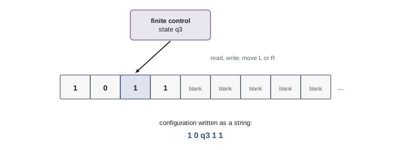
A configuration of M is a snapshot: the tape contents, the head position and the state. A standard notation writes it as a single string \(u\,q\,v\), meaning the tape holds uv followed by blanks, the machine is in state q, and the head is on the first symbol of v. One step takes a configuration to its successor, written \(C \vdash C'\). M accepts w if there is a finite sequence of configurations \(C_0 \vdash C_1 \vdash \cdots \vdash C_k\) starting in the initial configuration \(q_0 w\) and ending in an accepting configuration. This string representation of configurations, which turns a computation into a sequence of strings, is the key to several proofs later in the course, including the Cook–Levin theorem and the undecidability of problems about grammars.
Programming Turing machines
Writing Turing machines at the level of individual transitions is laborious but instructive, because it shows how much can be done with so little. The program below simulates single-tape machines and runs two of them. The first increments a binary number: it moves right to the end of the input, then moves left turning trailing 1s into 0s until it finds a 0 or a blank to turn into 1. The second decides the palindromes over \(\{a, b\}\), the language that no DFA can recognize. It crosses off the first symbol, remembering it in its state, runs to the last symbol, checks that it matches, crosses it off, and returns to the left end to repeat. The step counts grow roughly as \(n^2/2\), because each of about \(n/2\) round trips traverses the remaining string.
# A single-tape Turing machine simulator.
# delta[(state, symbol)] = (new_state, write, move) with move in "LR"; "_" is the blank.
def run(delta, w, start, accept, reject, max_steps=100_000):
    tape = dict(enumerate(w)); head, state, steps = 0, start, 0
    while state not in (accept, reject) and steps < max_steps:
        sym = tape.get(head, "_")
        if (state, sym) not in delta:
            state = reject; break
        state, tape[head], move = delta[(state, sym)]
        head += 1 if move == "R" else -1
        steps += 1
    lo, hi = min(tape, default=0), max(tape, default=0)
    out = "".join(tape.get(i, "_") for i in range(lo, hi + 1)).strip("_")
    return state, steps, out

# Binary increment: move right to the end, then add 1 with carries moving left.
INC = {("r", "0"): ("r", "0", "R"), ("r", "1"): ("r", "1", "R"), ("r", "_"): ("c", "_", "L"),
       ("c", "1"): ("c", "0", "L"), ("c", "0"): ("done", "1", "L"), ("c", "_"): ("done", "1", "L")}
for w in ["0", "1011", "111", "1001111"]:
    st, n, out = run(INC, w, "r", "done", "no")
    print(f"increment {w:>8} -> {out:>8}  ({n} steps)")

# Palindromes over {a, b}: cross off the first symbol, run to the last, compare, return.
PAL = {("s", "_"): ("acc", "_", "R"),
       ("s", "a"): ("ra", "_", "R"), ("s", "b"): ("rb", "_", "R")}
for x in "ab":
    for y in "ab": PAL[(f"r{x}", y)] = (f"r{x}", y, "R")
    PAL[(f"r{x}", "_")] = (f"c{x}", "_", "L")
    PAL[(f"c{x}", x)] = ("back", "_", "L")
    PAL[(f"c{x}", "_")] = ("acc", "_", "R")             # odd length: the middle symbol is gone
for y in "ab": PAL[("back", y)] = ("back", y, "L")
PAL[("back", "_")] = ("s", "_", "R")
for w in ["abba", "abab", "a" * 10, "ab" * 10 + "ba" * 10, "aab"]:
    st, n, _ = run(PAL, w, "s", "acc", "rej")
print(f"palindrome? {w[:22]:22s} n = {len(w):2d}: {st == 'acc'!s:5} steps {n:4d} steps/n^2 = {n / len(w) ** 2:.2f}")increment 0 -> 1 (3 steps) increment 1011 -> 1100 (8 steps) increment 111 -> 1000 (8 steps) increment 1001111 -> 1010000 (13 steps) palindrome? abba n = 4: True steps 15 steps/n^2 = 0.94 palindrome? abab n = 4: False steps 5 steps/n^2 = 0.31 palindrome? aaaaaaaaaa n = 10: True steps 66 steps/n^2 = 0.66 palindrome? ababababababababababba n = 40: True steps 861 steps/n^2 = 0.54 palindrome? aab n = 3: False steps 4 steps/n^2 = 0.44
Beyond a few dozen states, nobody writes Turing machines this way. Instead we describe them at higher levels. An implementation-level description says in prose how the head moves and what it writes, as in the palindrome description above. A high-level description gives an algorithm in ordinary language, such as 'mark the first unmarked node; repeat until no new nodes are marked: mark every node adjacent to a marked node; accept if the target is marked'. The Church–Turing thesis, discussed below, is what justifies treating such descriptions as Turing machines: we are confident that any clearly specified mechanical procedure could be compiled down to transitions, even though we never do it.
Variants are all equivalent
Many modifications of the model seem to add power, and none does. A multitape Turing machine has k tapes, each with its own head, and its transition depends on all k symbols under the heads. Theorem. Every multitape machine has an equivalent single-tape machine. The simulation stores the k tapes on one tape, separated by a delimiter, with a mark on each cell where a virtual head sits. To simulate one step, the single head sweeps across the tape to read the k marked symbols, then sweeps again to update them and move the marks, shifting parts of the tape right when a virtual tape grows. If the multitape machine runs for t steps, its tapes have length at most t, so each simulated step costs \(O(t)\), and the total is \(O(t^2)\): a quadratic slowdown. The program below compares the two approaches on a copying task and shows the ratio growing linearly with the input length.
# Simulating a two-tape machine on one tape costs at most a quadratic slowdown.
# Task: copy the input after a separator (w -> w#w). Count steps for a 2-tape strategy
# (read tape 1 and write tape 2 in one sweep, then write back) against a 1-tape strategy
# (shuttle back and forth, carrying one symbol per round trip).
def two_tape_steps(n):
    return n + 1 + n                      # one sweep copying to tape 2, one sweep appending

def one_tape_steps(w):
    tape = list(w) + ["#"]; steps = 0
    for i in range(len(w)):
        c = tape[i]; tape[i] = c.upper()   # mark the symbol being carried
        pos = i
        while pos < len(tape): pos += 1; steps += 1       # walk to the end
        tape.append(c); steps += 1                         # write it
        while pos > i: pos -= 1; steps += 1                # walk back to the mark
        steps += 1                                         # step past it
    return steps, "".join(tape).lower()

for n in [4, 8, 16, 32, 64, 128]:
    w = ("ab" * n)[:n]
    s1, out = one_tape_steps(w)
    s2 = two_tape_steps(n)
print(f"n = {n:3d}: two tapes {s2:5d} steps, one tape {s1:6d} steps, ratio {s1 / s2:6.1f} output ok: {out == w + '#' + w}")n = 4: two tapes 9 steps, one tape 48 steps, ratio 5.3 output ok: True n = 8: two tapes 17 steps, one tape 160 steps, ratio 9.4 output ok: True n = 16: two tapes 33 steps, one tape 576 steps, ratio 17.5 output ok: True n = 32: two tapes 65 steps, one tape 2176 steps, ratio 33.5 output ok: True n = 64: two tapes 129 steps, one tape 8448 steps, ratio 65.5 output ok: True n = 128: two tapes 257 steps, one tape 33280 steps, ratio 129.5 output ok: True
A nondeterministic Turing machine (NTM) has a transition relation instead of a function and accepts if some branch of its computation accepts. Theorem. Every NTM has an equivalent deterministic machine. The simulation explores the tree of computation branches breadth first, using a third tape to enumerate paths in the tree in order of length. Breadth-first rather than depth-first search matters: a depth-first search could follow an infinite branch forever and miss an accepting branch elsewhere. If the nondeterministic machine accepts in t steps along some branch, the simulation finds it after exploring at most \(b^{t}\) nodes, where b is the maximum number of choices per step, so the simulation is exponentially slower. Whether this exponential cost can be avoided for polynomial-time machines is exactly the P versus NP question of lesson 10.
Other variants fall the same way. Tapes infinite in both directions, a stay-put move, a two-dimensional grid of cells, several heads on one tape, a tape alphabet of only \(\{0, 1, \sqcup\}\), a machine with two stacks, a random-access machine with registers and indirect addressing, much like a real processor: each can be simulated by a single-tape Turing machine with at most a polynomial slowdown, and each can simulate one. An enumerator, a Turing machine with a printer that prints strings forever, gives another characterization: a language is Turing-recognizable if and only if some enumerator prints exactly its strings, possibly with repetitions and in any order.
| Variant | Simulation idea | Time cost of simulation |
|---|---|---|
| Multitape (k tapes) | Interleave tapes on one tape with head marks | Quadratic |
| Two-way infinite tape | Fold the tape in half onto two tracks | Linear |
| Nondeterministic | Breadth-first search of the computation tree | Exponential (best known) |
| Random-access machine | Store registers and memory on tapes with addresses | Polynomial |
| Two-stack PDA | One stack holds the left part of the tape, the other the right | Linear |
| Enumerator | Run the recognizer on all strings in dovetailed fashion | Same languages, no time bound |
| Binary tape alphabet | Encode each tape symbol as a fixed-length block of bits | Linear |
Encodings and universal machines
A Turing machine is a finite object, so it can be encoded as a string \(\langle M \rangle\): list its states, alphabets and transitions in some fixed format. Once machines are strings, machines can take other machines as input. Turing's most influential construction is the universal Turing machine U, which takes \(\langle M, w \rangle\) and simulates M on w, accepting if M accepts. U keeps M's description on one part of its tape and M's simulated tape on another, and at each step looks up the transition for the current state and symbol. Universality is the theoretical ancestor of the stored-program computer: one fixed machine that runs any program given as data. It also opens the door to self-reference, which is the engine of the undecidability proofs in the next lesson.
The Church–Turing thesis
In 1936 Alonzo Church proposed that the functions computable by the lambda calculus, which you met in CMPUT-325, are exactly the effectively calculable ones, and Turing independently proposed the same for his machines; the two models were quickly shown to be equivalent, as were Gödel and Herbrand's recursive functions and Post's systems. The Church–Turing thesis states that every function that can be computed by an algorithm, in the intuitive sense of a finite, mechanical, step-by-step procedure, can be computed by a Turing machine. It is a thesis rather than a theorem, because 'algorithm' in the intuitive sense is not a mathematical object. The evidence for it is strong: every proposed model of computation has turned out to be equivalent or weaker, Turing's analysis of what a human computer can do is persuasive, and no counterexample has emerged in ninety years.
The thesis is what turns results about Turing machines into results about all of computing. When we prove in lesson 8 that no Turing machine decides the halting problem, the thesis tells us that no program in Python, Rust or any future language decides it either, and no computer of any architecture. It is important to separate the thesis from stronger claims. The extended Church–Turing thesis says that every reasonable model can be simulated by a Turing machine with only polynomial overhead; quantum computers are the main challenge to it, as lesson 12 discusses. Neither thesis is threatened by speculative 'hypercomputers' that would perform infinitely many steps in finite time; none is known to be physically realizable.
Busy beavers: how complex small machines can be
How long can a small Turing machine run before halting? Define the busy beaver step function \(S(n)\) as the largest number of steps taken by any n-state, two-symbol machine that halts when started on a blank tape. Tibor Radó introduced the function in 1962 and proved that it grows faster than any computable function, so it is not computable: a machine computing S could be used to decide whether any machine halts on a blank tape, by running it for S(n) steps. Small values are known by exhaustive search with clever proofs that the non-halting machines never halt: \(S(2) = 6\), \(S(3) = 21\), \(S(4) = 107\). In July 2024 the collaborative bbchallenge project announced a proof, checked in the Coq proof assistant, that \(S(5) = 47{,}176{,}870\), settling a question open since the 1980s. For six states only enormous lower bounds are known, and some six-state machines encode open problems in number theory, so determining \(S(6)\) may be beyond current mathematics.
# Busy beavers: among halting n-state, 2-symbol machines started on a blank tape,
# the champions below take the most steps. Each one is simulated directly.
CHAMPS = {   # standard notation: for each state, the action on reading 0 then on reading 1
    2: "1RB1LB_1LA1RZ",
    3: "1RB1RZ_1LB0RC_1LC1LA",
    4: "1RB1LB_1LA0LC_1RZ1LD_1RD0RA",
}
def parse(code):
    d = {}
    for s, block in zip("ABCDE", code.split("_")):
        for sym, act in zip((0, 1), (block[:3], block[3:])):
            d[(s, sym)] = (int(act[0]), act[1], act[2])
    return d

def run(d, limit=10 ** 6):
    tape, head, state, steps = {}, 0, "A", 0
    while state != "Z" and steps < limit:
        w, mv, nxt = d[(state, tape.get(head, 0))]
        tape[head] = w; head += 1 if mv == "R" else -1; state = nxt; steps += 1
    return steps, sum(tape.values())

for n, code in CHAMPS.items():
    steps, ones = run(parse(code))
    print(f"n = {n}: champion {code:28s} halts after {steps:4d} steps with {ones:2d} ones")
print("n = 5: champion halts after 47,176,870 steps with 4,098 ones (BB(5), proved in 2024)")
print("n = 6: known lower bounds are astronomically large; the value is not known")n = 2: champion 1RB1LB_1LA1RZ halts after 6 steps with 4 ones n = 3: champion 1RB1RZ_1LB0RC_1LC1LA halts after 21 steps with 5 ones n = 4: champion 1RB1LB_1LA0LC_1RZ1LD_1RD0RA halts after 107 steps with 13 ones n = 5: champion halts after 47,176,870 steps with 4,098 ones (BB(5), proved in 2024) n = 6: known lower bounds are astronomically large; the value is not known
Worked examples
Worked problem
Implementation-level description
Describe a Turing machine that decides \(\{a^nb^nc^n : n \ge 0\}\).
Show solution
- Scan the input to check it has the form a*b*c*; reject otherwise.
- Return to the left end. Cross off one a, then move right and cross off one b, then one c. If any is missing, reject.
- Return to the left end and repeat until no a remains.
- Then scan once more: accept if no uncrossed b or c remains, otherwise reject.
Answer: A decider running in \(O(n^2)\) time, showing that this non-context-free language is decidable.
Worked problem
Reading a configuration
A machine is in configuration \(1\,0\,q_5\,1\,1\). The transition is \(\delta(q_5, 1) = (q_2, 0, L)\). What is the next configuration?
Show solution
- The head is on the third symbol, a 1, in state \(q_5\).
- It writes 0 there, moves left onto the second symbol, and enters q2.
- The tape now reads 1 0 0 1 and the head is on the second cell.
Answer: \(1\,q_2\,0\,0\,1\).
Worked problem
Cost of simulating multitape machines
A 3-tape machine runs in 1,000 steps. Roughly how many steps does the single-tape simulation take?
Show solution
- Each tape holds at most about 1,000 cells, so the combined tape has a few thousand cells.
- Each simulated step needs a constant number of sweeps over the tape, about c times 3,000 steps.
- Over 1,000 simulated steps that is on the order of 1,000 times 3,000, a few million steps.
Answer: On the order of \(10^6\) to \(10^7\) steps: quadratic in the original running time.
Common mistakes
MistakeTreat "the machine does not accept" as "the machine rejects".
InsteadA Turing machine may also run forever; recognizing and deciding are different.
MistakeUse depth-first search to simulate a nondeterministic machine.
InsteadAn infinite branch could trap the search; use breadth-first search.
MistakeCall the Church-Turing thesis a theorem.
InsteadIt links a formal model to an informal notion and cannot be proved, though the evidence is overwhelming.
MistakeAssume multitape machines decide more languages.
InsteadThey decide the same languages, only faster (at most quadratically).
MistakeThink busy beaver values can be computed for any n by running machines long enough.
InsteadS(n) grows faster than every computable function and is uncomputable in general.
Summary and key terms
- A Turing machine has a finite control and an unbounded tape it can read, write and move along in either direction.
- On each input a TM accepts, rejects or runs forever; deciders always halt.
- Turing-recognizable languages are accepted by some TM; decidable languages by some decider.
- Multitape, nondeterministic, random-access and other variants recognize the same languages.
- Multitape costs at most a quadratic slowdown to simulate; the best known simulation of nondeterminism is exponential.
- A universal TM simulates any machine given its description, the ancestor of the stored-program computer.
- The Church-Turing thesis identifies algorithms with Turing machines; BB(5) = 47,176,870 was proved in 2024.
- Turing machine
- A finite-state control with an unbounded read-write tape.
- Configuration
- A snapshot of tape contents, head position and state, often written u q v.
- Turing-recognizable
- Accepted by some Turing machine; also called recursively enumerable.
- Decidable
- Accepted by a Turing machine that halts on every input; also called recursive.
- Decider
- A Turing machine that halts on every input.
- Multitape Turing machine
- A Turing machine with several tapes and independent heads.
- Nondeterministic Turing machine
- A Turing machine with a transition relation that accepts if some branch accepts.
- Universal Turing machine
- A machine that simulates any machine given its encoding and input.
- Enumerator
- A Turing machine that prints the strings of a language.
- Church-Turing thesis
- The claim that every algorithm can be carried out by a Turing machine.
- Busy beaver
- The maximum number of steps of a halting n-state machine started on a blank tape.
Practice problems
Work each problem on paper first, then reveal the answer to check.
What are the three possible outcomes of running a TM on an input?
Show answer
Accept, reject, or run forever.
Why does simulating k tapes on one tape cost only a quadratic slowdown?
Show answer
After t steps each tape has length at most t, so each simulated step costs O(t) sweeps.
Why must the deterministic simulation of an NTM use breadth-first search?
Show answer
Depth-first search could follow an infinite branch and never find an accepting one.
Give a language that a TM decides but no PDA recognizes.
Show answer
\(\{a^nb^nc^n\}\).
What does a universal Turing machine take as input?
Show answer
An encoding \(\langle M, w \rangle\) of a machine and an input.
What is the busy beaver value S(4)?
Show answer
107 steps.
What does the extended Church-Turing thesis add?
Show answer
That simulation between reasonable models costs only polynomial overhead.
How does an enumerator characterize recognizable languages?
Show answer
A language is recognizable iff some enumerator prints exactly its strings.
Lesson quiz · 5 questions
Score 60% or more to complete this lesson.
Create a free account to save your progress, take quizzes and earn a certificate.