Time complexity: P, NP and NP-completeness

Computability theory separates the solvable from the unsolvable. Complexity theory asks, among solvable problems, which can be solved efficiently. The standard answer, proposed by Cobham and Edmonds in the mid-1960s, is that a problem is efficiently solvable if it can be decided in time bounded by a polynomial in the input length. The class of such problems is P. Many important problems are not known to be in P, but have a different, weaker property: a proposed solution can be checked in polynomial time. These form the class NP. Whether the two classes are equal is the P versus NP question. This lesson defines both classes, proves the Cook–Levin theorem that SAT is NP-complete, and builds a chain of reductions that makes many other problems NP-complete, extending the introduction in CMPUT-204 with full definitions and proofs.

Measuring running time

The running time of a decider M is the function \(t(n)\) giving the maximum number of steps M takes on any input of length n. We use asymptotic notation from CMPUT-204 and write \(\text{TIME}(t(n))\) for the class of languages decided by some single-tape Turing machine in \(O(t(n))\) time. The model matters for exact bounds: the palindrome language is in \(\text{TIME}(n^2)\) on one tape, and in fact needs \(\Omega(n^2)\) there, but takes linear time on two tapes. Lesson 7 showed that all reasonable deterministic models simulate each other with polynomial overhead, so the class \(\text{P} = \bigcup_k \text{TIME}(n^k)\) is the same for all of them. That robustness, together with the fact that polynomials are closed under composition, is why P is the standard formalization of 'efficiently solvable'.

P contains a great deal: graph reachability, shortest paths, minimum spanning trees, matching, linear programming, context-free parsing (lesson 5), primality testing (shown to be in P by Agrawal, Kayal and Saxena in 2002) and much more. Of course an \(n^{100}\) algorithm is not practical, and an exponential algorithm can beat a polynomial one for every input that fits on Earth. But in practice, problems that are shown to be in P usually soon get algorithms of low degree, and problems that resist polynomial algorithms usually resist them because of real combinatorial explosion. The polynomial boundary has proved a remarkably good guide.

The class NP

A verifier for a language A is an algorithm V such that \(A = \{w : V \text{ accepts } \langle w, c \rangle \text{ for some string } c\}\). The string c is a certificate or witness. A polynomial-time verifier runs in time polynomial in \(|w|\), which forces useful certificates to have polynomial length. Definition. NP is the class of languages that have polynomial-time verifiers. Equivalently, NP is the class of languages decided by nondeterministic Turing machines in polynomial time, \(\text{NP} = \bigcup_k \text{NTIME}(n^k)\): the nondeterministic machine guesses the certificate and runs the verifier, and conversely a certificate can record the choices of an accepting branch. The name means 'nondeterministic polynomial time', not 'non-polynomial'.

Examples abound. HAMPATH: does a graph have a path visiting every vertex exactly once? The certificate is the path. SUBSET-SUM: does some subset of given numbers sum to a target? The certificate is the subset. SAT: is a Boolean formula satisfiable? The certificate is a satisfying assignment. CLIQUE: does a graph have k mutually adjacent vertices? The certificate is the set of vertices. Every problem in P is in NP, because a verifier can ignore the certificate and solve the problem directly. The program below implements verifiers for three NP problems. Each is short, obviously polynomial, and needs only the certificate to confirm a yes answer; none of them helps with confirming a no answer, which is the asymmetry that the class coNP, discussed below, captures.

# NP as "quickly checkable": verifiers for three problems, each running in polynomial time.
# A verifier gets the instance and a proposed certificate, and checks it.
def verify_hampath(n, edges, path):
    E = {frozenset(e) for e in edges}
    return (sorted(path) == list(range(n))
            and all(frozenset((path[i], path[i + 1])) in E for i in range(n - 1)))

def verify_subset_sum(nums, target, chosen):
    return len(set(chosen)) == len(chosen) and all(0 <= i < len(nums) for i in chosen) \
        and sum(nums[i] for i in chosen) == target

def verify_sat(clauses, assign):
    return all(any((lit > 0) == assign[abs(lit)] for lit in c) for c in clauses)

edges = [(0, 1), (1, 2), (2, 3), (3, 4), (0, 2), (1, 4)]
print("Hamiltonian path 0-1-2-3-4:", verify_hampath(5, edges, [0, 1, 2, 3, 4]))
print("Hamiltonian path 0-2-1-4-3:", verify_hampath(5, edges, [0, 2, 1, 4, 3]))
print("Not a path      0-3-1-2-4:", verify_hampath(5, edges, [0, 3, 1, 2, 4]))
nums = [34, 4, 12, 5, 2, 27, 18]
print("subset {4, 12, 2, 18} sums to 36:", verify_subset_sum(nums, 36, [1, 2, 4, 6]))
cnf = [(1, -2, 3), (-1, 2), (2, -3), (-1, -2, -3)]
print("x1=T, x2=T, x3=F satisfies the formula:", verify_sat(cnf, {1: True, 2: True, 3: False}))
print("x1=T, x2=T, x3=T satisfies the formula:", verify_sat(cnf, {1: True, 2: True, 3: True}))

Hamiltonian path 0-1-2-3-4: True
Hamiltonian path 0-2-1-4-3: True
Not a path      0-3-1-2-4: False
subset {4, 12, 2, 18} sums to 36: True
x1=T, x2=T, x3=F satisfies the formula: True
x1=T, x2=T, x3=T satisfies the formula: False

Polynomial-time reductions and NP-completeness

Language A is polynomial-time reducible to B, written \(A \le_p B\), if there is a polynomial-time computable function f with \(w \in A \iff f(w) \in B\). This is a mapping reduction with a time bound. If \(A \le_p B\) and \(B \in \text{P}\), then \(A \in \text{P}\), because composing f with a polynomial-time decider for B is still polynomial. A language B is NP-hard if every language in NP reduces to it, and NP-complete if additionally \(B \in \text{NP}\). NP-complete problems are the hardest problems in NP: if any one of them is in P, then \(\text{P} = \text{NP}\), and if any problem in NP is not in P, then no NP-complete problem is in P. Reductions are transitive, so to show a new problem NP-complete, it suffices to show it is in NP and that some known NP-complete problem reduces to it.

The Cook–Levin theorem

Theorem (Cook, 1971; Levin, 1973). SAT is NP-complete. SAT is in NP, because an assignment is a certificate. For hardness, take any language A in NP, decided by a nondeterministic machine N in time \(n^k\). Given an input w of length n, we build in polynomial time a formula \(\phi_w\) that is satisfiable exactly when N has an accepting branch on w. The idea is a tableau: an \(n^k \times n^k\) table whose rows are the configurations of one branch, row i being the configuration at step i. Variables \(x_{i,j,s}\) say that cell \((i, j)\) contains symbol s, where symbols include tape symbols and states (configurations are written as strings, as in lesson 7, with the state written just before the head's cell).

The formula is a conjunction of four parts. \(\phi_{\text{cell}}\) says each cell contains exactly one symbol. \(\phi_{\text{start}}\) says the first row is the initial configuration on w. \(\phi_{\text{accept}}\) says some cell contains the accept state. \(\phi_{\text{move}}\) says each row follows from the previous one by a legal move. The key observation is that legality is local: a row follows legally from the one above if and only if every \(2 \times 3\) window of cells is consistent with N's transition function, and each window condition is a fixed-size formula over the variables of six cells. There are \(O(n^{2k})\) cells and windows, so \(\phi_w\) has polynomial size, and it can be written down in polynomial time. A satisfying assignment describes a valid accepting tableau, and an accepting branch gives a satisfying assignment.

The same proof gives more. With small changes the formula is in conjunctive normal form with at most three literals per clause, so 3SAT, satisfiability of such formulas, is also NP-complete. Any long clause \((\ell_1 \lor \ell_2 \lor \cdots \lor \ell_m)\) can be split into three-literal clauses with fresh variables, \((\ell_1 \lor \ell_2 \lor z_1) \land (\overline{z_1} \lor \ell_3 \lor z_2) \land \cdots\), preserving satisfiability. By contrast 2SAT, with two literals per clause, is in P, solvable by finding strongly connected components of an implication graph. The boundary between easy and hard can be very sharp.

A chain of reductions

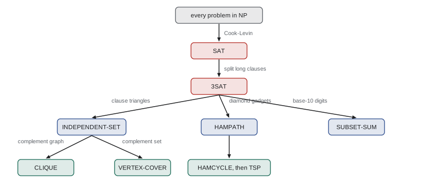
From 3SAT, reductions spread NP-completeness to thousands of problems. Richard Karp's 1972 paper showed 21 problems NP-complete, and Garey and Johnson's 1979 catalog listed several hundred. The figure shows a few links. Each reduction is a gadget construction that translates the structure of one problem into the other. The reduction from 3SAT to INDEPENDENT-SET is typical. For each clause, create a triangle of three vertices, labeled by the clause's literals; then join every vertex labeled x to every vertex labeled \(\overline{x}\). Ask for an independent set of size k, the number of clauses. An independent set can use at most one vertex per triangle, so it must use exactly one, which selects one true literal per clause, and the contradiction edges ensure the selected literals are consistent. The program below builds the graph for a small formula and checks the correspondence.

# The reduction from 3SAT to INDEPENDENT-SET, checked on small formulas.
# Each clause becomes a group of mutually joined literal-vertices; contradictory literals are joined.
# The formula is satisfiable iff the graph has an independent set of size k = number of clauses.
from itertools import combinations, product

def reduce(clauses):
    V = [(ci, pos, lit) for ci, c in enumerate(clauses) for pos, lit in enumerate(c)]
    E = set()
    for u, v in combinations(V, 2):
        if u[0] == v[0] or u[2] == -v[2]:
            E.add(frozenset({u, v}))
    return V, E, len(clauses)

def independent_sets(V, E, k):
    return [S for S in combinations(V, k) if all(frozenset({u, v}) not in E for u, v in combinations(S, 2))]

def satisfying(clauses):
    n = max(abs(l) for c in clauses for l in c)
    return [a for a in product([False, True], repeat=n)
            if all(any((l > 0) == a[abs(l) - 1] for l in c) for c in clauses)]

phi = [(1, 2, -3), (-1, -2, 3), (1, -2, -3), (-1, 2, 3)]
V, E, k = reduce(phi)
sets = independent_sets(V, E, k)
print(f"formula 1: {len(V)} vertices, {len(E)} edges, k = {k}")
print("  independent sets of size k:", len(sets), "  satisfying assignments:", len(satisfying(phi)))
S = sets[0]
assign = {abs(l): l > 0 for _, _, l in S}
print("  one set picks literals", [l for _, _, l in S], "-> assignment", assign)
print("  (several sets can give the same assignment when a clause has two true literals)")

psi = [(1, 2), (1, -2), (-1, 2), (-1, -2)]      # unsatisfiable; clauses of size 2 work the same way
V, E, k = reduce(psi)
print(f"formula 2: {len(V)} vertices, {len(E)} edges, k = {k}")
print("  independent sets of size k:", len(independent_sets(V, E, k)), "  satisfying assignments:", len(satisfying(psi)))

formula 1: 12 vertices, 24 edges, k = 4
  independent sets of size k: 14   satisfying assignments: 4
  one set picks literals [1, -2, 1, 3] -> assignment {1: True, 2: False, 3: True}
  (several sets can give the same assignment when a clause has two true literals)
formula 2: 8 vertices, 12 edges, k = 4
  independent sets of size k: 0   satisfying assignments: 0

The other links are similar in spirit. INDEPENDENT-SET reduces to CLIQUE by complementing the graph, since an independent set in G is a clique in its complement, and to VERTEX-COVER because S is independent exactly when the remaining vertices cover every edge. 3SAT reduces to HAMPATH by building, for each variable, a 'diamond' of vertices that can be traversed left to right (true) or right to left (false), with detours to clause vertices that can be taken only in the direction that makes the clause true. 3SAT reduces to SUBSET-SUM by writing numbers in base 10 with one digit per variable and per clause, so that choosing numbers corresponds to choosing literal values and the target forces each clause digit to be satisfied. HAMPATH reduces to the traveling salesperson problem by giving edges cost 1 and non-edges cost 2.

coNP and the shape of the landscape

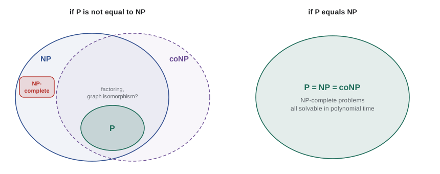
The class coNP contains the complements of NP languages: problems whose no answers have short certificates. TAUTOLOGY, whether a formula is true under every assignment, is coNP-complete; a falsifying assignment certifies a no answer, but no short certificate for a yes answer is known. Clearly \(\text{P} \subseteq \text{NP} \cap \text{coNP}\), and it is widely believed that \(\text{NP} \ne \text{coNP}\), which would imply \(\text{P} \ne \text{NP}\). Some problems lie in \(\text{NP} \cap \text{coNP}\) without being known to be in P: factoring (in its decision form) is one, because a factorization certifies both yes and no answers when combined with primality certificates. If \(\text{P} \ne \text{NP}\), Ladner's theorem (1975) guarantees problems in NP that are neither in P nor NP-complete; factoring and graph isomorphism are natural candidates. In 2015 László Babai announced a quasi-polynomial algorithm for graph isomorphism, placing it very close to P.

Pseudo-polynomial time

SUBSET-SUM is NP-complete, yet a simple dynamic program solves it in time \(O(nT)\) for n numbers and target T. There is no contradiction. The input encodes T in binary using about \(\log_2 T\) bits, so a running time polynomial in T is exponential in the input length. Such algorithms are called pseudo-polynomial, and problems that become easy when numbers are written in unary, like SUBSET-SUM and KNAPSACK, are called weakly NP-complete. Problems that remain NP-complete even with numbers bounded by a polynomial in the input length, such as 3-PARTITION and bin packing, are strongly NP-complete. The program below compares the work done by brute force and by the dynamic program. While the numbers are at most 1,000 the dynamic program does far less work; when the numbers grow to about \(2^n\), the number of distinct reachable sums explodes and the advantage shrinks, as the theory predicts. This is the encoding issue first raised in lesson 1, with real consequences.

# SUBSET-SUM: exponential brute force versus pseudo-polynomial dynamic programming.
# The DP does O(n * T) work: polynomial in the VALUE of T but exponential in its number of bits.
import random
from itertools import combinations
random.seed(474)

def brute(nums, T):
    # worst case: examine every subset (an early exit only helps on lucky yes-instances)
    examined, found = 0, False
    for r in range(len(nums) + 1):
        for c in combinations(nums, r):
            examined += 1
            found = found or sum(c) == T
    return found, examined

def dp(nums, T):
    reach = {0}; work = 0
    for x in nums:
        work += len(reach)
        reach |= {s + x for s in reach if s + x <= T}
    return T in reach, work

print(" n   max value        T   answer   subsets examined   DP work")
for n, top in ((12, 1000), (18, 1000), (22, 1000), (16, 2 ** 16), (20, 2 ** 20)):
    nums = [random.randint(1, top) for _ in range(n)]
    T = sum(nums) // 2 + 1
    (b, ex), (d, w) = brute(nums, T), dp(nums, T)
    assert b == d
    print(f"{n:2d}  {top:9d}  {T:9d}   {b!s:6s} {ex:17d}   {w:9d}")

 n   max value        T   answer   subsets examined   DP work
12       1000       3230   True                4096        2579
18       1000       3731   True              262144       21129
22       1000       5385   True             4194304       44568
16      65536     287017   False              65536       44141
20    1048576    5172851   False            1048576      665137

Living with NP-completeness

Proving a problem NP-complete is not the end of the story; it changes the question. If P differs from NP, there is no algorithm that is always fast and always exact. So one can give up 'always fast' and use exponential algorithms that are fast on the instances that occur, such as branch and bound, integer programming solvers or SAT solvers; give up 'always exact' and use approximation algorithms with proven guarantees or heuristics without them; or give up generality and exploit special structure, since many NP-complete problems are easy on trees, planar graphs or bounded parameters. The program below compares brute-force search with DPLL, the backtracking procedure with unit propagation at the core of modern SAT solvers, on random formulas near the hardest ratio of clauses to variables. Lesson 12 returns to why SAT solvers succeed on enormous industrial instances.

# Brute force versus DPLL (unit propagation and branching) on random 3-CNF formulas.
import random
random.seed(474)

def brute(n, clauses):
    tried = 0
    for m in range(2 ** n):
        tried += 1
        a = [(m >> i) & 1 == 1 for i in range(n)]
        if all(any((l > 0) == a[abs(l) - 1] for l in c) for c in clauses): return True, tried
    return False, tried

def dpll(clauses, assign, stats):
    stats[0] += 1
    changed = True
    while changed:                                    # unit propagation
        changed = False
        simplified = []
        for c in clauses:
            if any(assign.get(abs(l)) == (l > 0) for l in c): continue
            rest = [l for l in c if abs(l) not in assign]
            if not rest: return False
            if len(rest) == 1:
                assign[abs(rest[0])] = rest[0] > 0; changed = True
            simplified.append(rest)
        clauses = simplified
    if not clauses: return True
    x = abs(clauses[0][0])
    for val in (True, False):
        if dpll(clauses, {**assign, x: val}, stats): return True
    return False

def random_3cnf(n, m):
    return [tuple(random.choice([-1, 1]) * v for v in random.sample(range(1, n + 1), 3)) for _ in range(m)]

print(" n   clauses  sat?   brute-force assignments   DPLL nodes")
for n in (10, 14, 18, 22):
    f = random_3cnf(n, int(4.26 * n))                 # near the satisfiability threshold
    s1, t = brute(n, f)
    st = [0]; s2 = dpll(f, {}, st)
    print(f"{n:2d}   {len(f):5d}   {str(s2):5s}  {t:22d}   {st[0]:9d}")

 n   clauses  sat?   brute-force assignments   DPLL nodes
10      42   False                    1024          21
14      59   False                   16384          13
18      76   True                    68078           6
22      93   True                   819875          16

Worked examples