
CMPUT-291 · Lesson 2 of 12 · 32 min
The relational model and relational algebra
The relational model is the foundation under every SQL database. It describes all data as relations, which look like tables, and all queries as operations that take relations and produce new relations. Because the model is mathematical, it gives precise meanings to queries, lets a DBMS rewrite them into faster equivalent forms, and keeps the logical description of data separate from how it is stored. This lesson defines relations, keys and integrity constraints, then introduces relational algebra, the small set of operations from which every SQL query is built. The set theory and logic from CMPUT-272, especially sets, Cartesian products, relations and predicates, are used throughout.
Relations, tuples and attributes
In the relational model a database is a set of relations. A relation has a name and a set of attributes, each with a domain, the set of allowed values. A relation schema is written with its name and attributes, for example student(student_id, name, dept_id, credits). A relation instance is a set of tuples, each tuple assigning one value from the appropriate domain to each attribute. In table terms, the relation is the table, attributes are columns, and tuples are rows. The number of attributes is the degree of the relation; the number of tuples is its cardinality.
Formally, if the domains are \(D_1, D_2, \ldots, D_n\), a relation instance is a subset of the Cartesian product \(D_1 \times D_2 \times \cdots \times D_n\). This is exactly the definition of an n-ary relation from discrete mathematics, which is where the model gets its name. Two consequences follow directly from the set definition. A relation has no duplicate tuples, because a set contains each element once. And the tuples of a relation have no order: there is no first or last row. SQL relaxes both rules, as lesson 4 shows, but the model is cleaner with them.
| student_id | name | dept_id | credits |
|---|---|---|---|
| 101 | Ava | CS | 54 |
| 102 | Ben | CS | 30 |
| 103 | Chloe | MATH | 87 |
| 108 | Hiro | NULL | 0 |
Values in the relational model are atomic: each attribute value is a single, indivisible value from its domain, not a list or a nested table. A student with two phone numbers is therefore represented with a separate relation of phone numbers rather than a phone attribute holding a list. This requirement is called first normal form, and lesson 8 returns to it. Modern SQL systems do offer array and JSON types, and they are useful, but the classical theory, and good design in most cases, assumes atomic values.
Some values are unknown or do not apply: a student who has not chosen a department, an instructor whose salary is confidential. The relational model in SQL represents these with a special marker, NULL. NULL is not zero and not an empty string; it means 'no value here'. NULLs make comparisons three-valued, as lesson 4 explains, and are a frequent source of subtle errors. Good designs allow NULL only where it has a clear meaning.
Keys
A key identifies tuples. A superkey of a relation is a set of attributes whose values are different for every pair of distinct tuples, in every legal instance. A candidate key is a minimal superkey: removing any attribute from it would stop it being a superkey. A relation may have several candidate keys; the designer chooses one as the primary key and the others are alternate keys. In the student relation, {student_id} is a candidate key; {student_id, name} is a superkey but not a candidate key, because it is not minimal. If the college also guaranteed that every student had a unique email address, {email} would be a second candidate key.
Keys are statements about every legal instance, not observations about today's data. Today no two students may happen to share a name, but names are not a key because two students could share one tomorrow. Choosing keys is part of design, based on what the real world guarantees. Many designs use a surrogate key, an artificial identifier such as an integer assigned by the system, because natural keys like names and even government identifiers can change, be missing or be reused.
from itertools import combinations

# A small instance; which attribute sets uniquely identify rows HERE?
rows = [
    {"sid": 101, "name": "Ava",   "email": "ava@x.ca",   "dept": "CS"},
    {"sid": 102, "name": "Ben",   "email": "ben@x.ca",   "dept": "CS"},
    {"sid": 103, "name": "Chloe", "email": "chloe@x.ca", "dept": "MATH"},
    {"sid": 104, "name": "Ava",   "email": "ava2@x.ca",  "dept": "BIO"},
]
attrs = list(rows[0])

def unique(cols):
    vals = [tuple(r[c] for c in cols) for r in rows]
    return len(set(vals)) == len(vals)

supers = [set(c) for k in range(1, len(attrs) + 1) for c in combinations(attrs, k) if unique(c)]
minimal = [s for s in supers if not any(t < s for t in supers)]
print("superkeys in this instance:", len(supers))
print("minimal ones:", [sorted(s) for s in minimal])superkeys in this instance: 13 minimal ones: [['sid'], ['email'], ['dept', 'name']]
The code finds {dept, name} unique in this small instance, but no college would accept that as a key: two students with the same name could join the same department. Data can show that something is not a key, because one counterexample is enough, but it can never prove that something is a key. That decision belongs to the designer.
Integrity constraints
Integrity constraints are conditions every legal instance must satisfy. The DBMS checks them on every change and rejects changes that would violate them. The relational model has three basic kinds. Domain constraints require each value to come from the attribute's domain, for example credits being a non-negative integer. Key constraints require candidate key values to be unique; entity integrity additionally requires primary key attributes to be non-NULL, since a tuple must be identifiable. Referential integrity requires that a foreign key, a set of attributes in one relation that refers to the primary key of another, either matches an existing tuple or is NULL.
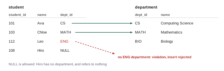
In the college database used throughout this course, student.dept_id is a foreign key referring to department.dept_id. Inserting a student with dept_id 'ENG' would fail if no ENG department exists, and deleting the CS department would fail, or cascade, while students still refer to it. Lesson 3 shows how SQL declares these constraints and the options for what happens on delete.
Relational algebra: the operations
Relational algebra is a set of operations on relations. Each operation takes one or two relations and produces a new relation, so operations can be composed into expressions, just as arithmetic operations compose into formulas. This closure property is what makes the algebra powerful. A DBMS translates every SQL query into an algebra expression, then rewrites that expression into an equivalent one that is cheaper to evaluate. Knowing the algebra therefore explains what SQL means and why the optimizer can do what it does.
| Operation | Symbol | Result | SQL counterpart |
|---|---|---|---|
| Selection | \(\sigma_{p}(R)\) | Tuples of R satisfying predicate p | WHERE |
| Projection | \(\pi_{A}(R)\) | R restricted to attributes A, duplicates removed | SELECT DISTINCT column list |
| Union | \(R \cup S\) | Tuples in R or S (same schema) | UNION |
| Difference | \(R - S\) | Tuples in R but not S | EXCEPT |
| Intersection | \(R \cap S\) | Tuples in both | INTERSECT |
| Cartesian product | \(R \times S\) | Every pairing of a tuple of R with a tuple of S | FROM R, S or CROSS JOIN |
| Rename | \(\rho_{T}(R)\) | R with a new name (or renamed attributes) | AS |
| Natural join | \(R \bowtie S\) | Pairs agreeing on all common attributes, shared columns once | NATURAL JOIN |
| Theta join | \(R \bowtie_{\theta} S\) | \(\sigma_{\theta}(R \times S)\) | JOIN ... ON condition |
Selection, written \(\sigma\) (sigma), picks the tuples that satisfy a condition, keeping all attributes: \(\sigma_{credits \geq 50}(student)\) gives students with at least 50 credits. Projection, written \(\pi\) (pi), keeps chosen attributes and discards the rest: \(\pi_{name}(student)\) gives the set of names. Because relations are sets, projection removes duplicates: if two students are named Ava, the result contains 'Ava' once. Selection cuts a table horizontally; projection cuts it vertically.
Union, difference and intersection are the set operations. They require union-compatible operands: the same number of attributes with compatible domains. Cartesian product pairs every tuple of one relation with every tuple of the other; if R has m tuples and S has n, \(R \times S\) has \(m \times n\). Product on its own is rarely what you want, but followed by a selection that matches related tuples it becomes a join, the most important operation of all. Rename, written \(\rho\) (rho), gives a relation or its attributes new names, which is needed when a relation is joined with itself.
Joins
A join combines related tuples from two relations. The theta join \(R \bowtie_{\theta} S\) is defined as \(\sigma_{\theta}(R \times S)\): form every pair, then keep the pairs that satisfy the condition \(\theta\). When the condition is an equality, such as student.dept_id = department.dept_id, it is an equijoin. The natural join \(R \bowtie S\) is an equijoin on all attributes with the same name, with the duplicate columns kept only once. Joins are how the relational model reassembles information that design has deliberately spread across tables.
student = [  # (student_id, name, dept_id)
    (101, "Ava", "CS"), (103, "Chloe", "MATH"), (105, "Elena", "BIO"), (108, "Hiro", None)]
department = [  # (dept_id, dept_name)
    ("CS", "Computing Science"), ("MATH", "Mathematics"), ("HIST", "History")]

def select(rel, pred):            return [t for t in rel if pred(t)]
def project(rel, idx):            return sorted(set(tuple(t[i] for i in idx) for t in rel))
def product(r, s):                return [a + b for a in r for b in s]

pairs = product(student, department)
print("product size:", len(student), "x", len(department), "=", len(pairs))
joined = select(pairs, lambda t: t[2] == t[3])           # equijoin on dept_id
print("join:", project(joined, (1, 4)))
cs_or_math = select(student, lambda t: t[2] in ("CS", "MATH"))
print("selection then projection:", project(cs_or_math, (1,)))product size: 4 x 3 = 12
join: [('Ava', 'Computing Science'), ('Chloe', 'Mathematics')]
selection then projection: [('Ava',), ('Chloe',)]The join drops two kinds of tuples. Hiro, whose department is NULL, matches no department because NULL equals nothing, not even NULL. The History department, which has no students in this fragment, matches no student. Sometimes those unmatched tuples matter: a report of every department and its students should list History with nobody. Outer joins, introduced in lesson 4, keep unmatched tuples and fill the missing side with NULLs.
Worked problem
Writing a query in relational algebra
Using student(student_id, name, dept_id, credits) and department(dept_id, name, building, budget), write an algebra expression for the names of students in departments located in Central Hall.
Show solution
- The building is in department, the student names in student; they are related through dept_id, so a join is needed.
- Select the relevant departments first: \(\sigma_{building = \text{Central Hall}}(department)\).
- Both relations have an attribute called name, so project department to dept_id before joining, avoiding a clash: \(\pi_{dept\_id}(\sigma_{building = \text{Central Hall}}(department))\).
- Natural join with student on dept_id, then project the student names.
- \[\pi_{name}\left(student \bowtie \pi_{dept\_id}\left(\sigma_{building = \text{Central Hall}}(department)\right)\right)\]
Answer: The expression above. With the college data it returns Chloe, Isla and Farid, the students in Mathematics and Physics.
Composing and rewriting expressions
Because every operation returns a relation, expressions can be nested and rearranged. Many rewrites are guaranteed to give the same result, and a query optimizer uses them to find cheaper plans. Selections can be pushed down below joins, so that tuples are filtered before they are paired; a sequence of selections can be combined or reordered; projections can be pushed down to drop unneeded columns early; joins are commutative and associative, so the optimizer can choose the order. These equivalences come from set theory and predicate logic, and they are why a declarative language can be fast.
Worked problem
Why pushing selections down helps
student has 20,000 tuples and enrollment has 300,000. A query wants the enrollments of the 400 students in the History department. Compare the number of pairs examined by (a) joining first and selecting afterwards with a naive nested loop, and (b) selecting History students first.
Show solution
- (a) A naive nested-loop join compares every student with every enrollment: \(20{,}000 \times 300{,}000 = 6 \times 10^{9}\) pairs, then filters.
- (b) Selecting first leaves 400 students. Joining them with enrollments compares \(400 \times 300{,}000 = 1.2 \times 10^{8}\) pairs.
- The ratio is \(6 \times 10^{9} / 1.2 \times 10^{8} = 50\). With an index on enrollment.student_id, case (b) would examine only the matching enrollments.
Answer: Pushing the selection down examines 50 times fewer pairs. Real optimizers apply such rewrites automatically, which lesson 9 explores.
Further operations
Several useful operations can be expressed with the basic ones but are given their own symbols. Division \(R \div S\) answers 'for all' questions, such as students who have taken every required course; it can be written using projection, product and difference, and SQL expresses it with nested NOT EXISTS, as lesson 5 shows. Extended relational algebra adds grouping and aggregation, written \(\gamma\) (gamma), to compute sums, counts and averages per group, and outer joins. SQL also works with bags (multisets) rather than sets, so that duplicates are kept unless DISTINCT is requested, because removing duplicates costs time and because counting duplicates is often what is wanted.
Relational algebra is procedural in the sense that an expression describes an order of operations. Relational calculus, the other formal query language Codd proposed, is declarative: it describes the result as a set defined by a logical formula, such as 'the set of names n such that there exists a student tuple with name n and credits at least 50'. Codd proved that the two have the same expressive power, a property called relational completeness. SQL borrows its SELECT-FROM-WHERE shape from the calculus and its operations from the algebra.
Common mistakes
MistakeTreating a value that is unique today as a key.
InsteadA key must be unique in every legal instance. Data can disprove a key with one duplicate but can never prove one; keys come from real-world rules.
MistakeCalling {student_id, name} a candidate key.
InsteadIt is a superkey but not minimal, because {student_id} alone is a key. A candidate key is a minimal superkey.
MistakeExpecting a join to keep tuples with no match.
InsteadInner joins drop unmatched tuples, including those with NULL in the join attribute. Use an outer join to keep them.
MistakeUsing union or difference on relations with different attributes.
InsteadSet operations require union-compatible relations with the same number of attributes and compatible domains.
MistakeForgetting that projection removes duplicates in the algebra.
InsteadRelations are sets, so \(\pi_{name}\) returns each name once. SQL keeps duplicates unless you write DISTINCT.
Summary and key terms
- A relation is a set of tuples over named attributes with domains; it is a subset of the Cartesian product of the domains, so it has no duplicates and no order.
- Values are atomic; NULL marks a missing or inapplicable value and is not equal to anything.
- A superkey uniquely identifies tuples; a candidate key is a minimal superkey; one candidate key is chosen as the primary key.
- Integrity constraints include domain, key, entity integrity and referential integrity; foreign keys must match an existing primary key value or be NULL.
- Relational algebra operations, selection, projection, set operations, product, rename and joins, take relations and return relations, so they compose.
- A theta join is a selection over a product; a natural join matches all common attribute names; inner joins drop unmatched tuples.
- Algebraic equivalences such as pushing selections below joins let optimizers evaluate declarative queries efficiently.
- Relation
- A named set of tuples over a fixed set of attributes; shown as a table.
- Tuple
- One element of a relation, assigning a value to each attribute; a row.
- Attribute
- A named column of a relation, with a domain of allowed values.
- Superkey
- A set of attributes whose values uniquely identify a tuple in every legal instance.
- Candidate key
- A minimal superkey.
- Primary key
- The candidate key chosen to identify tuples; its attributes may not be NULL.
- Foreign key
- Attributes in one relation whose values must match the primary key of another relation or be NULL.
- Selection
- The algebra operation \(\sigma\) that keeps tuples satisfying a condition.
- Projection
- The algebra operation \(\pi\) that keeps chosen attributes and removes duplicate tuples.
- Natural join
- A join that matches tuples on all attributes with the same name and keeps each shared attribute once.
Practice problems
Work each problem on paper first, then reveal the answer to check.
A relation has attributes (isbn, title, author, year) and 3,200 tuples. State its degree and cardinality.
Show answer
Degree 4 (attributes) and cardinality 3,200 (tuples).
Why can a relation in the formal model not contain two identical tuples?
Show answer
Because a relation is a set, and a set contains each element at most once.
In employee(emp_id, sin, name, dept), both emp_id and sin are unique. List the candidate keys and one superkey that is not a candidate key.
Show answer
Candidate keys {emp_id} and {sin}; {emp_id, name} is a superkey that is not minimal.
Which constraint is violated by inserting an enrollment for student 999 when no such student exists?
Show answer
Referential integrity: enrollment.student_id is a foreign key that must match an existing student.
If R has 40 tuples and S has 25, how many tuples does \(R \times S\) have?
Show answer
1,000.
Write an algebra expression for the names of courses worth 4 credits in course(course_id, title, dept_id, credits).
Show answer
\(\pi_{title}(\sigma_{credits = 4}(course))\).
What is the difference between an equijoin and a natural join?
Show answer
An equijoin uses an explicit equality condition and keeps both columns; a natural join equates all same-named attributes and keeps one copy of each.
Why does a student with a NULL dept_id not appear in student joined with department on dept_id?
Show answer
NULL is not equal to any value, so the join condition is never true for that tuple.
State one algebraic equivalence a query optimizer might use and why it helps.
Show answer
Pushing a selection below a join, \(\sigma_p(R \bowtie S) = \sigma_p(R) \bowtie S\) when p mentions only R, reduces the number of tuples the join must process.
What kind of question is relational division designed to answer?
Show answer
"For all" questions, such as students who have taken every course in a required set.
Lesson quiz · 5 questions
Score 60% or more to complete this lesson.
Create a free account to save your progress, take quizzes and earn a certificate.