
CMPUT-204 · Lesson 9 of 12 · 27 min
Shortest paths
Breadth-first search finds routes with the fewest edges, but real networks have edges of different lengths: roads have distances and travel times, network links have latencies, and flights have prices. This lesson finds shortest paths in weighted graphs. Dijkstra's algorithm handles non-negative weights in \(O((n + m)\log n)\) time and is the workhorse behind route planners. Bellman–Ford handles negative weights and detects negative cycles, at a higher cost. For DAGs, a single pass in topological order solves the problem in linear time and also finds the longest paths used in project scheduling.
The single-source shortest-path problem
In a weighted directed graph, each edge \((u, v)\) has a weight \(w(u, v)\), and the weight of a path is the sum of its edge weights. The distance \(\delta(s, v)\) is the minimum weight of a path from \(s\) to \(v\), or infinity if \(v\) is unreachable. The single-source problem asks for \(\delta(s, v)\) for every vertex \(v\), together with the paths. An undirected road can be modeled as two directed edges, one each way. Shortest paths have optimal substructure: any part of a shortest path is itself a shortest path between its endpoints, because a shorter part could be swapped in to shorten the whole path.
Negative weights need care. They arise naturally, for example as rebates in a cost network or as logarithms of exchange rates. If a cycle reachable from \(s\) has negative total weight, going around it repeatedly makes paths arbitrarily cheap, so shortest paths are undefined for vertices reachable from that cycle. Algorithms must either forbid negative weights or detect negative cycles.
Relaxation
All the algorithms in this lesson maintain an estimate \(d[v]\) of the distance to each vertex, starting with \(d[s] = 0\) and \(d[v] = \infty\) for all others, and a parent pointer for each vertex. The single operation that improves estimates is relaxation of an edge \((u, v)\): if going through \(u\) gives a shorter route to \(v\), take it.
Relaxation never makes an estimate wrong in the dangerous direction: every \(d[v]\) is always the weight of some actual path, so \(d[v] \ge \delta(s, v)\) at all times. The algorithms differ only in which edges they relax and in what order. Relax the right edges in the right order and every estimate falls to the true distance.
Dijkstra's algorithm
Dijkstra's algorithm, published by Edsger Dijkstra in 1959, works for graphs with non-negative edge weights. It grows a set \(S\) of vertices whose distances are final. At each step it chooses the vertex \(u\) outside \(S\) with the smallest estimate \(d[u]\), adds it to \(S\), and relaxes every edge leaving \(u\). With all weights non-negative, the smallest estimate outside \(S\) is guaranteed to be exact, so the algorithm never needs to revisit a vertex. It is a greedy algorithm, a design technique lesson 11 studies in general.
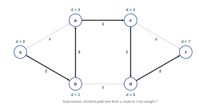
Why is the chosen vertex's estimate exact? Suppose \(u\) is chosen but some shorter path \(P\) from \(s\) to \(u\) exists. \(P\) starts inside \(S\) and must leave \(S\) at some edge \((x, y)\), with \(x \in S\) and \(y\) outside. Since \(x\)'s distance is final and its edges were relaxed, \(d[y] \le \delta(s, x) + w(x, y)\), which is at most the weight of \(P\) because the rest of \(P\) after \(y\) has non-negative weight. So \(d[y] \le w(P) < d[u]\), contradicting the choice of \(u\) as the vertex with the smallest estimate. The argument fails exactly when the rest of \(P\) could have negative weight.
import heapq

def dijkstra(adj, s):
    dist = {s: 0}
    parent = {s: None}
    done = set()
    pq = [(0, s)]                        # (estimate, vertex)
    pops = 0
    while pq:
        du, u = heapq.heappop(pq); pops += 1
        if u in done:
            continue                     # stale entry: lazy deletion
        done.add(u)
        for v, w in adj[u]:
            nd = du + w
            if v not in dist or nd < dist[v]:
                dist[v] = nd
                parent[v] = u
                heapq.heappush(pq, (nd, v))
    return dist, parent, pops

def route(parent, t):
    out = []
    while t is not None:
        out.append(t); t = parent[t]
    return out[::-1]

adj = {'s': [('a', 4), ('b', 1)], 'a': [('c', 1)], 'b': [('a', 2), ('d', 5)],
       'c': [('d', 1), ('t', 6)], 'd': [('t', 2)], 't': []}
dist, parent, pops = dijkstra(adj, 's')
print('distances:', dict(sorted(dist.items())))
print('route to t:', ' -> '.join(route(parent, 't')), 'weight', dist['t'])
print('heap pops:', pops)distances: {'a': 3, 'b': 1, 'c': 4, 'd': 5, 's': 0, 't': 7}
route to t: s -> b -> a -> c -> d -> t weight 7
heap pops: 9The route to \(t\) is s, b, a, c, d, t with weight 7, longer in edges than the direct-looking s, b, d, t but lighter, which BFS would get wrong. The code uses a common trick: rather than decreasing a key inside the heap, which heapq does not support, it pushes a new entry and skips stale ones when popped. Each edge causes at most one push, so the heap holds at most \(m\) entries and each operation costs \(O(\log m) = O(\log n)\).
| Priority queue | Extract-min | Decrease-key | Dijkstra total |
|---|---|---|---|
| Unsorted array | Θ(n) | Θ(1) | Θ(n²), best for dense graphs |
| Binary heap (or heapq with lazy deletion) | O(log n) | O(log n) | O((n + m) log n) |
| Fibonacci heap | O(log n) amortized | O(1) amortized | O(m + n log n) |
Worked problem
Tracing Dijkstra
Trace the first three selections of Dijkstra from s on the graph in the code above.
Show solution
- Start: d[s] = 0, all others ∞. Select s; relax s→a (4) and s→b (1).
- Select b (d = 1); relax b→a: 1 + 2 = 3 < 4, so d[a] = 3; relax b→d: d[d] = 6.
- Select a (d = 3); relax a→c: d[c] = 4.
- Next would be c (4), which improves d[d] to 5 and sets d[t] = 10; then d (5) improves d[t] to 7.
Answer: Selections s, b, a, then c, d, t, with final distances 0, 1, 3, 4, 5 and 7.
Negative weights and Bellman–Ford
With a negative edge, Dijkstra can finalize a vertex too early. In the graph with edges \(s \to a\) of weight 2, \(s \to b\) of weight 5 and \(b \to a\) of weight \(-4\), Dijkstra finalizes \(a\) at distance 2, but the path through \(b\) costs 1. The Bellman–Ford algorithm avoids any greedy choice. It relaxes every edge, in any order, \(n - 1\) times. After round \(i\), every vertex whose shortest path uses at most \(i\) edges has its correct distance, by induction on \(i\). Since a shortest path without cycles has at most \(n - 1\) edges, \(n - 1\) rounds suffice, for a total of \(\Theta(nm)\) time.
Bellman–Ford also detects negative cycles. After \(n - 1\) rounds, run one more pass over the edges. If any edge can still be relaxed, some estimate is still falling, which can only happen if a negative cycle is reachable from \(s\). This makes Bellman–Ford the standard tool for detecting arbitrage in currency markets: with edge weights \(-\log(\text{rate})\), a cycle of trades that multiplies money corresponds to a cycle of negative total weight. Distance-vector routing protocols, such as RIP on older networks, are distributed versions of Bellman–Ford.
import heapq, math

def bellman_ford(vertices, edges, s):
    d = {v: math.inf for v in vertices}
    d[s] = 0
    for _ in range(len(vertices) - 1):
        changed = False
        for u, v, w in edges:
            if d[u] + w < d[v]:
                d[v] = d[u] + w; changed = True
        if not changed:
            break                         # early exit: estimates are final
    cycle = any(d[u] + w < d[v] for u, v, w in edges)
    return d, cycle

def dijkstra_dist(vertices, edges, s):
    adj = {v: [] for v in vertices}
    for u, v, w in edges:
        adj[u].append((v, w))
    d, done, pq = {s: 0}, set(), [(0, s)]
    while pq:
        du, u = heapq.heappop(pq)
        if u in done: continue
        done.add(u)
        for v, w in adj[u]:
            if v not in done and du + w < d.get(v, math.inf):
                d[v] = du + w; heapq.heappush(pq, (d[v], v))
    return d

V = ['s', 'a', 'b']
E = [('s', 'a', 2), ('s', 'b', 5), ('b', 'a', -4)]
print('Dijkstra    :', dijkstra_dist(V, E, 's'))
print('Bellman-Ford:', bellman_ford(V, E, 's'))

rates = {('CAD', 'USD'): 0.73, ('USD', 'EUR'): 0.92, ('EUR', 'CAD'): 1.50}   # illustrative rates
cur = ['CAD', 'USD', 'EUR']
E2 = [(a, b, -math.log(r)) for (a, b), r in rates.items()]
print('product of rates around the cycle:', round(0.73 * 0.92 * 1.50, 4))
print('negative cycle (arbitrage)?', bellman_ford(cur, E2, 'CAD')[1])Dijkstra : {'s': 0, 'a': 2, 'b': 5}
Bellman-Ford: ({'s': 0, 'a': 1, 'b': 5}, False)
product of rates around the cycle: 1.0074
negative cycle (arbitrage)? TrueDijkstra reports a distance of 2 to \(a\), which is wrong; Bellman–Ford finds 1. The illustrative exchange rates multiply to a little more than 1 around the cycle, so converting money around it would make a small profit, and Bellman–Ford reports the corresponding negative cycle. Real markets close such gaps within milliseconds, and transaction fees usually erase them.
Shortest and longest paths in a DAG
If the graph is a DAG, there is an even simpler method. Topologically sort the vertices, as in lesson 8, and relax the edges leaving each vertex in that order. When a vertex is processed, every edge into it has already been relaxed, so its estimate is final. This takes \(\Theta(n + m)\) time and works with negative weights, since a DAG has no cycles at all.
Negating every weight turns the same method into a longest-path algorithm, which is otherwise a hard problem in general graphs. In project scheduling, tasks are vertices or edges of a DAG weighted by their durations, and the longest path from start to finish is the critical path: the minimum time to complete the project, and the chain of tasks where any delay delays everything. The critical path method used in construction planning, as in CON-210, is exactly this computation.
def dag_longest(order, adj, dur):
    """Earliest finish times; tasks given in topological order."""
    start = {t: 0 for t in order}
    via = {t: None for t in order}
    for u in order:
        for v in adj[u]:
            if start[u] + dur[u] > start[v]:     # relax for the longest path
                start[v] = start[u] + dur[u]
                via[v] = u
    finish = {t: start[t] + dur[t] for t in order}
    end = max(finish, key=finish.get)
    path, t = [], end
    while t is not None:
        path.append(t); t = via[t]
    return finish[end], path[::-1]

dur = {'design': 5, 'permits': 10, 'foundation': 7, 'framing': 12, 'electrical': 6, 'plumbing': 5, 'finish': 8}
adj = {'design': ['permits', 'foundation'], 'permits': ['framing'], 'foundation': ['framing'],
       'framing': ['electrical', 'plumbing'], 'electrical': ['finish'], 'plumbing': ['finish'], 'finish': []}
order = ['design', 'permits', 'foundation', 'framing', 'electrical', 'plumbing', 'finish']
length, path = dag_longest(order, adj, dur)
print('project length:', length, 'days')
print('critical path :', ' -> '.join(path))project length: 41 days critical path : design -> permits -> framing -> electrical -> finish
| Algorithm | Graph restriction | Time | Negative cycle detection |
|---|---|---|---|
| BFS | Unweighted (all weights equal) | Θ(n + m) | Not applicable |
| DAG relaxation in topological order | Acyclic | Θ(n + m) | Not applicable (no cycles) |
| Dijkstra with a binary heap | Non-negative weights | O((n + m) log n) | No |
| Bellman–Ford | Any weights | Θ(nm) | Yes |
For distances between every pair of vertices, running Dijkstra from each vertex costs \(O(n(n + m)\log n)\) on non-negative graphs, while the Floyd–Warshall algorithm, a dynamic-programming method covered in CMPUT-304, handles any weights in \(\Theta(n^3)\). Route planners for continental road networks go further, precomputing shortcuts so a query touches only a few thousand vertices out of millions; robot path planners in ROB-340 use A*, a Dijkstra variant guided by a distance estimate to the goal.
Common mistakes
MistakeUsing BFS on a weighted graph.
InsteadBFS minimizes the number of edges, not total weight; use Dijkstra for non-negative weights.
MistakeRunning Dijkstra on a graph with negative edges.
InsteadIt can finalize a vertex too early; use Bellman–Ford, or DAG relaxation if the graph is acyclic.
MistakeFinalizing a vertex when it is first pushed onto the heap.
InsteadA vertex is final only when popped with the smallest estimate; later pushes may improve it before then.
MistakeRunning Bellman–Ford for n rounds and ignoring a change in the last round.
Insteadn − 1 rounds suffice; any relaxation in an extra round signals a reachable negative cycle.
MistakeAssuming longest paths are as easy as shortest paths in any graph.
InsteadLongest simple paths are hard in general graphs; they are easy only in DAGs.
Summary and key terms
- Shortest paths minimize total edge weight; any part of a shortest path is itself shortest.
- Relaxation lowers an estimate d[v] when a route through u is shorter; estimates never go below true distances.
- Dijkstra repeatedly finalizes the closest unfinished vertex and is correct for non-negative weights.
- With a binary heap, Dijkstra runs in O((n + m) log n); heapq with lazy deletion achieves this in Python.
- Bellman–Ford relaxes all edges n − 1 times, handles negative weights in Θ(nm) and detects negative cycles.
- In a DAG, relaxing edges in topological order gives shortest paths in Θ(n + m), even with negative weights.
- Longest paths in a DAG give the critical path of a project schedule.
- Weighted graph
- A graph whose edges carry numbers such as lengths or costs.
- Distance
- The minimum total weight of a path from s to v, written δ(s, v).
- Relaxation
- Updating d[v] to d[u] + w(u, v) when that is smaller.
- Optimal substructure
- The property that parts of optimal solutions are themselves optimal.
- Dijkstra's algorithm
- A greedy single-source shortest-path algorithm for non-negative weights.
- Lazy deletion
- Leaving outdated heap entries in place and skipping them when they are popped.
- Bellman–Ford algorithm
- Relaxing every edge n − 1 times; works with negative weights.
- Negative cycle
- A cycle whose edge weights sum to less than zero.
- Critical path
- The longest path through a project DAG, which determines the minimum completion time.
- Arbitrage
- A cycle of exchanges that returns more than it started with, a negative cycle under −log weights.
Practice problems
Work each problem on paper first, then reveal the answer to check.
Relax edge (u, v) with d[u] = 7, w = 3, d[v] = 12. What happens?
Show answer
d[v] becomes 10 and parent[v] becomes u.
Why can Dijkstra stop considering a vertex once it is popped?
Show answer
With non-negative weights, the smallest estimate outside the finished set is exact, so it can never improve.
What is the running time of Bellman–Ford on 1,000 vertices and 5,000 edges, roughly?
Show answer
About 999 × 5,000 ≈ 5 million relaxations, Θ(nm).
Can a shortest path contain a positive-weight cycle?
Show answer
No; removing the cycle would give a shorter path.
What does Bellman–Ford conclude if an edge can be relaxed in round n?
Show answer
A negative cycle is reachable from the source.
Rates CAD→USD 0.74, USD→CAD 1.35. Is there arbitrage on this two-currency cycle?
Show answer
0.74 × 1.35 = 0.999 < 1, so no.
Why does DAG relaxation work with negative weights?
Show answer
Processing in topological order means all edges into a vertex are relaxed before it is used, and there are no cycles.
In the project example, which task could be delayed without delaying the project?
Show answer
Foundation (or plumbing), since it is not on the critical path design → permits → framing → electrical → finish.
Which priority queue makes Dijkstra Θ(n²), and when is that a good choice?
Show answer
An unsorted array; good for dense graphs where m is close to n².
Why is A* faster than Dijkstra for a single destination?
Show answer
It uses an estimate of the remaining distance to explore toward the goal first, settling fewer vertices.
Lesson quiz · 5 questions
Score 60% or more to complete this lesson.
Create a free account to save your progress, take quizzes and earn a certificate.