
CMPUT-204 · Lesson 4 of 12 · 26 min
Sorting I: elementary sorts and merge sort
Sorting is the most studied problem in algorithms, for good reasons. It is useful on its own, it is a first step in many other algorithms, such as the duplicate check in lesson 1 and Kruskal's algorithm in lesson 10, and it shows almost every design technique in a small space. This lesson studies two simple quadratic sorts, selection sort and insertion sort, and then merge sort, the first divide-and-conquer algorithm in the course, which sorts in \(\Theta(n \log n)\) time. Along the way it introduces the vocabulary used to compare sorting algorithms: comparisons, inversions, stability and extra space.
The sorting problem and how we measure sorts
The input is a sequence of \(n\) items, each with a key drawn from a totally ordered set, and the output is a permutation of the input with keys in non-decreasing order. The algorithms in this lesson and the next only learn about keys by comparing two of them, so they are called comparison sorts, and we usually count key comparisons as the basic operation. Two other properties matter in practice. A sort is in place if it uses only \(O(1)\) extra memory beyond the input array, or \(O(\log n)\) for a recursion stack. A sort is stable if items with equal keys keep their original relative order, which matters when you sort records by one field after another.
| Algorithm | Worst case | Best case | Extra space | Stable |
|---|---|---|---|---|
| Selection sort | Θ(n²) | Θ(n²) | Θ(1) | No (usual array version) |
| Insertion sort | Θ(n²) | Θ(n) | Θ(1) | Yes |
| Merge sort | Θ(n log n) | Θ(n log n) | Θ(n) | Yes |
| Quicksort (lesson 5) | Θ(n²) | Θ(n log n) | Θ(log n) expected | No |
| Heapsort (lesson 5) | Θ(n log n) | Θ(n log n) | Θ(1) | No |
Selection sort
Selection sort repeatedly finds the smallest remaining item and swaps it into place. After pass \(i\), positions 0 to \(i\) hold the \(i+1\) smallest items in order, which is the loop invariant. Finding the minimum of the \(n - i\) remaining items takes \(n - i - 1\) comparisons, so the total is \((n-1) + (n-2) + \cdots + 1 = n(n-1)/2\), whatever the input. Selection sort is therefore \(\Theta(n^2)\) in every case. Its one virtue is that it makes at most \(n - 1\) swaps, which matters only when moving items is far more expensive than comparing them.
Insertion sort
Insertion sort builds a sorted prefix one item at a time. It takes the next item and shifts larger items in the prefix one position right until it finds where the new item belongs, the way many people sort a hand of cards. Its invariant is that before processing position \(i\), the prefix \(a[0..i-1]\) contains the original first \(i\) items in sorted order. Insertion sort is stable, in place, simple, and very fast on small or nearly sorted inputs, which is why production sorting routines use it for short runs.
def insertion_sort(a):
    a = list(a)
    comps = shifts = 0
    for i in range(1, len(a)):
        key = a[i]
        j = i - 1
        while j >= 0:
            comps += 1
            if a[j] <= key:          # <= keeps equal keys in order: stable
                break
            a[j + 1] = a[j]          # shift right
            shifts += 1
            j -= 1
        a[j + 1] = key
    return a, comps, shifts

def inversions_brute(a):
    return sum(1 for i in range(len(a)) for j in range(i + 1, len(a)) if a[i] > a[j])

import random
random.seed(204)
n = 200
cases = {'sorted': list(range(n)), 'reversed': list(range(n, 0, -1)),
         'random': random.sample(range(n), n)}
for name, data in cases.items():
    out, c, s = insertion_sort(data)
    assert out == sorted(data)
print(f'{name:>8}: comparisons {c:>6}, shifts {s:>6}, inversions {inversions_brute(data):>6}')sorted: comparisons 199, shifts 0, inversions 0 reversed: comparisons 19900, shifts 19900, inversions 19900 random: comparisons 9753, shifts 9561, inversions 9561
The output reveals the exact cost of insertion sort. The number of shifts always equals the number of inversions in the input, where an inversion is a pair of positions \(i < j\) with \(a[i] > a[j]\). Each shift swaps one adjacent out-of-order pair and so removes exactly one inversion. A sorted list has no inversions and needs \(n - 1\) comparisons; a reversed list has the maximum \(n(n-1)/2\) inversions. A random permutation has, on average, half of all pairs inverted, \(n(n-1)/4\), so the average case is also \(\Theta(n^2)\). That argument proves something stronger: any sort that only swaps adjacent items, including bubble sort, needs \(\Omega(n^2)\) swaps on average.
Worked problem
Counting inversions by hand
How many inversions does 3, 1, 4, 2 have, and how many shifts will insertion sort make?
Show solution
- List the out-of-order pairs: (3, 1), (3, 2), (4, 2).
- The pair (1, 4) and (1, 2) and (3, 4) are in order.
- So there are 3 inversions.
- Insertion sort will shift exactly 3 times: 1 past 3, then 2 past 4 and past 3.
Answer: 3 inversions and 3 shifts. The number of inversions measures how far a list is from sorted.
Merge sort: divide and conquer
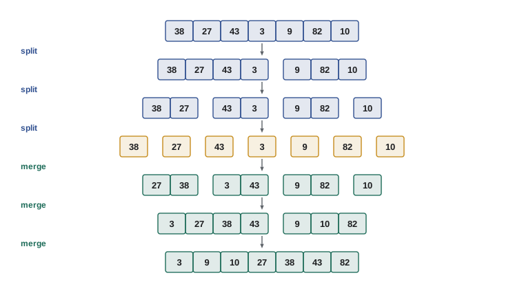
Merge sort follows the divide-and-conquer pattern from lesson 3. Divide the list into two halves. Conquer by sorting each half recursively. Combine by merging the two sorted halves into one sorted list. A list of length 0 or 1 is already sorted, which is the base case. All the real work happens in the merge step.
To merge two sorted lists \(L\) and \(R\), keep a pointer at the front of each. Repeatedly compare the two front items, move the smaller one to the output and advance its pointer. When one list runs out, append the rest of the other. Each comparison outputs one item, and the last item is output without a comparison, so merging lists of total length \(n\) takes at most \(n - 1\) comparisons. Taking from the left list when the keys are equal makes merge sort stable.
def merge(left, right, counter):
    out = []
    i = j = 0
    while i < len(left) and j < len(right):
        counter[0] += 1
        if left[i] <= right[j]:          # take from the left on ties: stable
            out.append(left[i]); i += 1
        else:
            out.append(right[j]); j += 1
    out.extend(left[i:])
    out.extend(right[j:])
    return out

def merge_sort(a, counter):
    if len(a) <= 1:
        return list(a)
    mid = len(a) // 2
    return merge(merge_sort(a[:mid], counter), merge_sort(a[mid:], counter), counter)

import math, random
random.seed(4)
print(merge_sort([38, 27, 43, 3, 9, 82, 10], [0]))
for n in (2**10, 2**14, 2**17):
    data = [random.random() for _ in range(n)]
    c = [0]
    assert merge_sort(data, c) == sorted(data)
print(n, c[0], round(n * math.log2(n)), round(c[0] / (n * math.log2(n)), 3))[3, 9, 10, 27, 38, 43, 82] 1024 8929 10240 0.872 16384 208469 229376 0.909 131072 2062401 2228224 0.926
On random inputs merge sort uses about \(n \log_2 n - 1.25n\) comparisons, which is 87 to 93 percent of \(n \log_2 n\) for these sizes and creeps toward 100 percent as \(n\) grows. The saving comes from merges that end with one list exhausted early. The worst case is at most \(n \lceil \log_2 n \rceil - n + 1\) comparisons, and even the best case, an already sorted list, needs about half of \(n \log_2 n\), because each merge still compares until one side runs out. Unlike insertion sort, merge sort does not adapt much to sorted input.
Why merge sort is correct
Correctness follows by strong induction on the length \(n\). Lists of length 0 or 1 are sorted, so the base case returns a correct result. For \(n \ge 2\), both halves are shorter than \(n\), so by the inductive hypothesis the recursive calls return them sorted. The merge then produces a sorted list containing exactly the items of both halves, by its own loop invariant: the output holds the smallest items seen so far in sorted order, and the front items of \(L\) and \(R\) are the smallest remaining ones in their lists. So merge sort returns a sorted permutation of its input.
Analysis and space
The running time satisfies \(T(n) = 2T(n/2) + \Theta(n)\), which lesson 3 solved with a recursion tree and the master theorem: \(T(n) \in \Theta(n \log n)\). This holds in every case, because the splitting does not depend on the data. The price is memory. The straightforward version creates new lists at every level, but even a careful array implementation needs a temporary buffer of \(n\) items for merging, so merge sort uses \(\Theta(n)\) extra space. In-place merging is possible but complicated and slow, which is one reason quicksort and heapsort, studied next, remain important.
Worked problem
Counting comparisons in a small merge
Merge L = [2, 5, 9] and R = [3, 4, 10, 12]. How many comparisons are made?
Show solution
- Compare 2 and 3: output 2. Compare 5 and 3: output 3. Compare 5 and 4: output 4.
- Compare 5 and 10: output 5. Compare 9 and 10: output 9.
- L is now empty, so 10 and 12 are appended without comparisons.
- That is 5 comparisons for 7 items, fewer than the maximum of 6.
Answer: 5 comparisons. A merge uses at most n − 1 comparisons and stops early when one list empties.
Bottom-up merge sort and other variations
Merge sort need not be recursive. Bottom-up merge sort treats the input as \(n\) runs of length 1, merges adjacent pairs into runs of length 2, then 4, and so on, doubling the run length on each pass. There are \(\lceil \log_2 n \rceil\) passes, each costing \(\Theta(n)\), giving the same \(\Theta(n \log n)\) bound without any recursion. Natural merge sort goes further and starts from the runs already present in the data, so nearly sorted input needs very few passes. Python's built-in sort, Timsort, uses this idea together with insertion sort for short runs, which makes it \(\Theta(n)\) on already sorted data and \(\Theta(n \log n)\) in the worst case.
Merge sort is also the algorithm of choice for data that does not fit in memory. External merge sort reads chunks that fit in RAM, sorts each one, writes the sorted runs to disk and then merges many runs at once with a priority queue (lesson 5). Each pass reads and writes the data sequentially, which suits disks and networked storage far better than the random access other sorts need.
Counting inversions with merge sort
The number of inversions measures how different two rankings are, for example two people's rankings of the same films. Counting them by checking all pairs takes \(\Theta(n^2)\) time. A small change to merge sort counts them in \(\Theta(n \log n)\). During a merge, whenever an item from the right half is output before items remaining in the left half, it forms an inversion with every one of those remaining left items, because they are larger and came earlier. Adding that count at each step totals the inversions that cross between the halves; the recursive calls count those within each half.
def sort_count(a):
    """Return (sorted list, number of inversions) in Theta(n log n) time."""
    if len(a) <= 1:
        return list(a), 0
    mid = len(a) // 2
    left, x = sort_count(a[:mid])
    right, y = sort_count(a[mid:])
    out, i, j, cross = [], 0, 0, 0
    while i < len(left) and j < len(right):
        if left[i] <= right[j]:
            out.append(left[i]); i += 1
        else:
            out.append(right[j]); j += 1
            cross += len(left) - i       # right[j] precedes all remaining left items
    out += left[i:] + right[j:]
    return out, x + y + cross

import random
random.seed(7)
print(sort_count([3, 1, 4, 2])[1])
data = random.sample(range(2000), 2000)
fast = sort_count(data)[1]
slow = sum(1 for i in range(len(data)) for j in range(i + 1, len(data)) if data[i] > data[j])
print(fast, slow, fast == slow)3 998169 998169 True
The count for 3, 1, 4, 2 agrees with the hand calculation above, and on 2,000 random items the fast method matches the brute-force count. The random count is close to the expected \(n(n-1)/4 \approx 999{,}500\). Recommendation systems use exactly this measure, often normalized as Kendall's tau, to compare rankings.
Common mistakes
MistakeClaiming insertion sort is Θ(n²) in every case.
InsteadIts running time is Θ(n + I), where I is the number of inversions: Θ(n) when sorted, Θ(n²) in the worst and average cases.
MistakeUsing < instead of <= when merging and calling the result stable.
InsteadTake from the left list on equal keys; otherwise equal items can change order.
MistakeSaying merge sort is in place.
InsteadArray merge sort needs a Θ(n) buffer; only complicated variants avoid it.
MistakeExpecting merge sort to be fast on already sorted input.
InsteadTop-down merge sort still makes Θ(n log n) comparisons; natural merge sort and Timsort exploit existing runs.
MistakeCounting only the inversions found inside each half.
InsteadAdd the cross inversions found during the merge, len(left) − i each time a right item is taken first.
Summary and key terms
- Comparison sorts learn about keys only by comparing them; we count comparisons and also note stability and extra space.
- Selection sort makes n(n − 1)/2 comparisons on every input but at most n − 1 swaps.
- Insertion sort runs in Θ(n + I), where I is the number of inversions, so it is fast on nearly sorted data.
- Merging two sorted lists of total length n takes at most n − 1 comparisons.
- Merge sort satisfies T(n) = 2T(n/2) + Θ(n), so it runs in Θ(n log n) in every case, using Θ(n) extra space.
- Merge sort is stable, parallelizes well and suits external sorting of data on disk.
- A modified merge counts inversions in Θ(n log n) instead of Θ(n²).
- Comparison sort
- A sorting algorithm that gains information only by comparing pairs of keys.
- Stable sort
- A sort that keeps items with equal keys in their original relative order.
- In-place sort
- A sort that uses only O(1), or O(log n) stack, extra memory.
- Inversion
- A pair of positions i < j with a[i] > a[j].
- Selection sort
- Repeatedly select the minimum of the unsorted part and swap it into place.
- Insertion sort
- Insert each item into its place in a growing sorted prefix by shifting larger items.
- Merge
- Combine two sorted lists into one sorted list by repeatedly taking the smaller front item.
- Merge sort
- Divide and conquer: sort each half recursively, then merge.
- Run
- A maximal sorted stretch of consecutive items.
- External sorting
- Sorting data too large for main memory by sorting chunks and merging runs from disk.
Practice problems
Work each problem on paper first, then reveal the answer to check.
How many comparisons does selection sort make on 50 items?
Show answer
50 × 49 / 2 = 1,225, on every input.
How many inversions does 5, 4, 3, 2, 1 have?
Show answer
10, the maximum for 5 items: 5 × 4 / 2.
Insertion sort is run on a list with 12 inversions and 100 items. About how many comparisons?
Show answer
About n − 1 + I = 99 + 12 = 111 (each shift costs one comparison plus one stopping comparison per item).
Merge [1, 6, 7] and [2, 3, 8]. How many comparisons?
Show answer
5: 1|2, 6|2, 6|3, 6|8, 7|8, then 8 is appended.
Why is insertion sort used for short runs inside fast library sorts?
Show answer
It has very low overhead and is Θ(n) on nearly sorted data, so it beats Θ(n log n) methods for small n.
What is the depth of merge sort's recursion for n = 1,024?
Show answer
log₂ 1024 = 10 levels of splitting below the root.
Give an input where an unstable sort produces a different output from a stable one.
Show answer
Records (2, a), (1, b), (2, c) sorted by number: a stable sort keeps (2, a) before (2, c); an unstable sort may swap them.
How many passes does bottom-up merge sort make on 1,000 items?
Show answer
⌈log₂ 1000⌉ = 10 passes.
Why does adjacent swapping need Ω(n²) swaps on average?
Show answer
Each adjacent swap removes at most one inversion and a random permutation has n(n − 1)/4 inversions on average.
During a merge, left = [5, 8, 9] with i = 0 and the next item taken is 4 from the right. How many cross inversions are added?
Show answer
3, since 4 precedes 5, 8 and 9.
Lesson quiz · 5 questions
Score 60% or more to complete this lesson.
Create a free account to save your progress, take quizzes and earn a certificate.