Fixed-priority scheduling and response-time analysis

Almost every real-time operating system schedules tasks by fixed priority: each task is given a priority when it is created, and at every instant the processor runs the highest-priority task that is ready. The rule is simple to implement, cheap at run time and easy to reason about, and it degrades gracefully, because when the system is overloaded it is the lowest-priority tasks that suffer first. What it does not do by itself is guarantee deadlines. That needs two further ingredients: a sensible way to assign the priorities, and a test that proves, for the chosen priorities, that every task meets its deadline. This lesson develops both, from the famous utilization bound of Liu and Layland to the exact response-time analysis that is the workhorse of industrial timing verification.

Jonah now has the NS-5 task table from lesson 2. Maren Holt's question at the design review is direct: with the kernel's fixed-priority scheduler, will every task always meet its deadline, and how much room is there for the features marketing wants to add next year?

Assigning priorities

The rate-monotonic (RM) rule gives higher priority to tasks with shorter periods. For the NS-5 this means RADAR (6.25 ms) highest, then CANTX (10 ms), CLASS (25 ms), LOG (100 ms) and HOUSE (1,000 ms) lowest. Liu and Layland proved in 1973 that, for independent periodic tasks with implicit deadlines on one processor, rate-monotonic priority assignment is optimal among fixed-priority assignments: if any fixed-priority assignment meets all deadlines, rate-monotonic does too.

When deadlines are shorter than periods, the deadline-monotonic (DM) rule, which gives higher priority to tasks with shorter relative deadlines, is optimal instead, as Leung and Whitehead showed in 1982. For implicit deadlines the two rules coincide. Neither rule is optimal once tasks have release jitter combined with arbitrary deadlines, or share resources in complex ways. For those cases Audsley's optimal priority assignment algorithm works from the bottom: it tries to find some task that is schedulable at the lowest priority with all others above it, fixes it there, and repeats for the next level up. It needs at most n(n + 1)/2 schedulability tests and finds a feasible assignment whenever one exists for tests with the right properties.

Priorities should reflect timing, not importance. A tempting mistake is to give the most important task the highest priority, regardless of its period. If the NS-5's housekeeping task, which reads the battery voltage and is important to the product's survival, were given top priority, its 20 ms of execution would delay a radar frame by up to 20 ms and cause a string of missed frames. The task with the 1,000 ms period has 980 ms of slack and does not need priority to meet its deadline. Importance matters when the system is overloaded, and lesson 8 deals with that separately through mixed-criticality scheduling.

The Liu and Layland utilization bound

The first schedulability test is a sufficient condition based only on utilization. Liu and Layland proved that a set of n independent periodic tasks with implicit deadlines is schedulable under rate-monotonic priorities if its total utilization satisfies:

The bound is 1 for one task, 0.828 for two, 0.780 for three, 0.757 for four and 0.743 for five, and it falls toward ln 2, about 0.693, as n grows. Any task set under the bound is schedulable, regardless of the individual periods. A task set over the bound may still be schedulable, because the bound is derived from the worst possible combination of periods. Harmonic task sets, in which each period divides every longer one, are schedulable under rate-monotonic priorities up to U = 1.

In 2003 Bini, Buttazzo and Buttazzo found a tighter test using the same information, the hyperbolic bound. A task set is schedulable under rate-monotonic priorities if:

The hyperbolic bound accepts every task set the Liu and Layland bound accepts, and some that it rejects. Both tests are fast and need no knowledge of the periods themselves, which makes them useful for quick design checks and for admission control at run time, but both are only sufficient. When they fail, the exact test is response-time analysis.

Response-time analysis

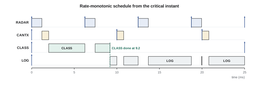
Response-time analysis computes the worst-case response time R_i of each task directly and compares it with the deadline. It was developed by Joseph and Pandya in 1986 and extended by Audsley, Burns, Richardson, Tindell and Wellings in the early 1990s. The key observation, due to Liu and Layland, is that a task's worst case occurs at the critical instant, when it is released at the same time as every higher-priority task. From that instant, the task's response time consists of its own execution time plus the interference from higher-priority tasks that are released before it finishes. A higher-priority task τ_j released every T_j preempts τ_i ceil(R_i/T_j) times during an interval of length R_i, each time taking C_j. The response time is therefore the smallest positive solution of:

where hp(i) is the set of tasks with higher priority than τ_i. R_i appears on both sides, so the equation is solved by fixed-point iteration. Start with R_i^(0) = C_i and compute each new value from the previous one:

The sequence never decreases. If two successive values are equal, that value is the worst-case response time. If a value exceeds the deadline D_i, the task is unschedulable and the iteration can stop. For constrained deadlines the test is exact: a task set is schedulable under the given priorities if and only if R_i ≤ D_i for every task. The iteration converges for every task whose higher-priority utilization is below 1, and in practice it takes only a handful of steps.

The code below applies both utilization tests and response-time analysis to the NS-5 task set, and then to a variant in which the classifier grows from 6 ms to 11 ms, which is what the planned pedestrian-detection feature is expected to cost. Times are kept in integer microseconds so that the ceiling function is exact; a floating-point value such as 25.000000001 would otherwise round up to an extra preemption.

from math import ceil, prod

def check(tasks):
    n = len(tasks)
    U = sum(c / t for _, c, t, _ in tasks)
    ll = n * (2 ** (1 / n) - 1)
    hyp = prod(c / t + 1 for _, c, t, _ in tasks)
    print(f"U = {U:.3f}   Liu-Layland bound for n = {n}: {ll:.4f}   "
          f"{'pass' if U <= ll else 'inconclusive'}")
    print(f"hyperbolic product = {hyp:.3f}   {'pass' if hyp <= 2 else 'inconclusive'}")

def rta(tasks):
    """tasks in priority order, highest first; times in microseconds"""
    for i, (name, c, t, d) in enumerate(tasks):
        r, steps = c, [c]
        while True:
            nxt = c + sum(ceil(r / tj) * cj for _, cj, tj, _ in tasks[:i])
            if nxt == r or nxt > d:
                break
            r = nxt
            steps.append(r)
        r = nxt
        trail = " -> ".join(f"{s/1000:g}" for s in steps)
        print(f"  {name:6s} R = {r/1000:5.1f} ms  D = {d/1000:g} ms  "
              f"{'met' if r <= d else 'MISSED'}   iterations: {trail}")

base = [("RADAR", 1_200, 6_250, 6_250), ("CANTX", 800, 10_000, 10_000),
        ("CLASS", 6_000, 25_000, 25_000), ("LOG", 8_000, 100_000, 100_000),
        ("HOUSE", 20_000, 1_000_000, 1_000_000)]
print("base task set")
check(base)
rta(base)

heavy = [(n, 11_000 if n == "CLASS" else c, t, d) for n, c, t, d in base]
print("CLASS with C = 11 ms")
check(heavy)
rta(heavy)

base task set
U = 0.612   Liu-Layland bound for n = 5: 0.7435   pass
hyperbolic product = 1.759   pass
  RADAR  R =   1.2 ms  D = 6.25 ms  met   iterations: 1.2
  CANTX  R =   2.0 ms  D = 10 ms  met   iterations: 0.8 -> 2
  CLASS  R =   9.2 ms  D = 25 ms  met   iterations: 6 -> 8 -> 9.2
  LOG    R =  21.2 ms  D = 100 ms  met   iterations: 8 -> 17.2 -> 19.2 -> 20.4 -> 21.2
  HOUSE  R =  64.8 ms  D = 1000 ms  met   iterations: 20 -> 40.4 -> 52.4 -> 61.6 -> 63.6 -> 64.8
CLASS with C = 11 ms
U = 0.812   Liu-Layland bound for n = 5: 0.7435   inconclusive
hyperbolic product = 2.042   inconclusive
  RADAR  R =   1.2 ms  D = 6.25 ms  met   iterations: 1.2
  CANTX  R =   2.0 ms  D = 10 ms  met   iterations: 0.8 -> 2
  CLASS  R =  16.2 ms  D = 25 ms  met   iterations: 11 -> 15 -> 16.2
  LOG    R =  42.4 ms  D = 100 ms  met   iterations: 8 -> 22.2 -> 26.2 -> 38.4 -> 41.6 -> 42.4
  HOUSE  R =  99.2 ms  D = 1000 ms  met   iterations: 20 -> 45.4 -> 63.6 -> 79.8 -> 94 -> 99.2

For the base task set, U = 0.612 is below the five-task bound of 0.7435, so the Liu and Layland test alone proves schedulability, and the hyperbolic product of 1.759 confirms it. Response-time analysis adds the actual margins: RADAR 1.2 ms, CANTX 2.0 ms, CLASS 9.2 ms, LOG 21.2 ms and HOUSE 64.8 ms, all well within their deadlines.

With the classifier at 11 ms, U rises to 0.812, above the bound, and the hyperbolic product of 2.042 exceeds 2, so both quick tests are inconclusive. They do not say the set is unschedulable; they simply cannot decide. Response-time analysis gives the answer: CLASS finishes within 16.2 ms of its release, LOG within 42.4 ms and HOUSE within 99.2 ms. Every deadline is still met. This is the typical industrial pattern: quick tests for early sizing, exact analysis for the sign-off.

How much room is left?

Schedulability is a yes-or-no answer; designers also want to know how much margin there is. Two measures are common. The breakdown utilization scales all execution times by a common factor until the set becomes unschedulable, and reports the utilization at that point. The critical scaling factor is the factor itself. For the NS-5 base set, a binary search around response-time analysis finds a critical scaling factor of about 1.63: every execution time can grow by 60 % before any deadline is at risk. At that point the utilization is almost exactly 1, which is unusually high for fixed priorities and comes from the nearly harmonic periods of 6.25, 25, 100 and 1,000 ms. A second, more targeted measure asks how much a single task can grow: sensitivity analysis on CLASS alone shows the maximum classifier execution time that keeps every task schedulable. Both are found by binary search around the response-time test, and both are standard features of commercial timing analysis tools. Margins like these should be part of every design review, because execution times grow as features are added and compilers change.

Extending the analysis

The basic equation assumes zero release jitter, no blocking and negligible overheads. Each assumption can be relaxed by adding a term. If a task can be released up to J_i after its nominal arrival, for example because it is released by a polled timer or a message that arrives with variable delay, a higher-priority task with jitter J_j can preempt more often than its period suggests, and the response time measured from the nominal arrival includes the task's own jitter:

Here B_i is the blocking term, the longest time τ_i can be delayed by lower-priority tasks holding shared resources, which lesson 7 computes. Kernel overheads such as context switches and the timer tick can be added to each C_j or modeled as extra high-priority tasks, as lesson 6 shows. For arbitrary deadlines longer than the period, the analysis must consider several jobs in a level-i busy period, because an earlier job of the same task can delay a later one; Lehoczky's 1990 extension handles this by iterating over each job in the busy period.

Fixed priority in practice

Fixed-priority scheduling with response-time analysis is the standard method in automotive control units, avionics partitions, industrial controllers and many medical devices. Its attractions go beyond the analysis. Overload behavior is predictable: if CLASS overruns, it can delay only LOG and HOUSE, never RADAR or CANTX. Priorities map directly onto the hardware interrupt controller, so interrupt handlers and tasks can be analyzed with the same equation, interrupts simply being the highest-priority tasks. And priority levels are a natural place to document design intent.

Its limitation is utilization. In the worst case, rate-monotonic scheduling cannot use the last 26 % or so of the processor while guaranteeing all deadlines, although for most real task sets the breakdown utilization is closer to 88 %, as Lehoczky, Sha and Ding showed for randomly generated sets in 1989. Lesson 5 introduces earliest deadline first, which can use the whole processor, and compares the two.