
CMP-440 · Lesson 12 of 12 · 22 min
Verification, safety standards and capstone design
A real-time system is finished not when it runs but when there is convincing evidence that it meets its timing requirements, along with its functional and safety requirements, under every condition it was designed for. That evidence comes from a combination of analysis, testing, review and monitoring, organized by a development process and, for safety-related systems, by an industry standard that says what evidence is needed and how much. This final lesson surveys verification methods for real-time systems, outlines the main functional safety standards and their integrity levels, explains how timing evidence fits into a safety case, and then brings the course together in the NS-5 timing sign-off.
The NS-5 is about to go to its first customer pilot, forty intersections for the Michigan Department of Transportation and the City of Ann Arbor. The pilot contract requires the vehicle-detection function to be developed to a recognized functional safety standard, and Maren Holt has asked Jonah to present the complete timing argument at the final design review, with hardware lead Ines Carvalho, field technician Dev Okafor and Dana Okoye from the server team in the room.
The V-model and where timing fits
Most safety-related development follows some form of the V-model. The left side descends from requirements through architecture and detailed design to code; the right side ascends through unit, integration and system verification, each level checking the corresponding level on the left. Timing appears at every level. Requirements state deadlines, periods and end-to-end limits with their sources, as lesson 1 described. The architecture fixes tasks, priorities, partitions, networks and the task table of lesson 2. Detailed design adds resource sharing and protocols. Unit verification produces WCET bounds and high-water marks. Integration verification runs schedulability analysis on the integrated task set with measured overheads and blocking. System verification measures end-to-end latency on the real hardware under worst-case load.
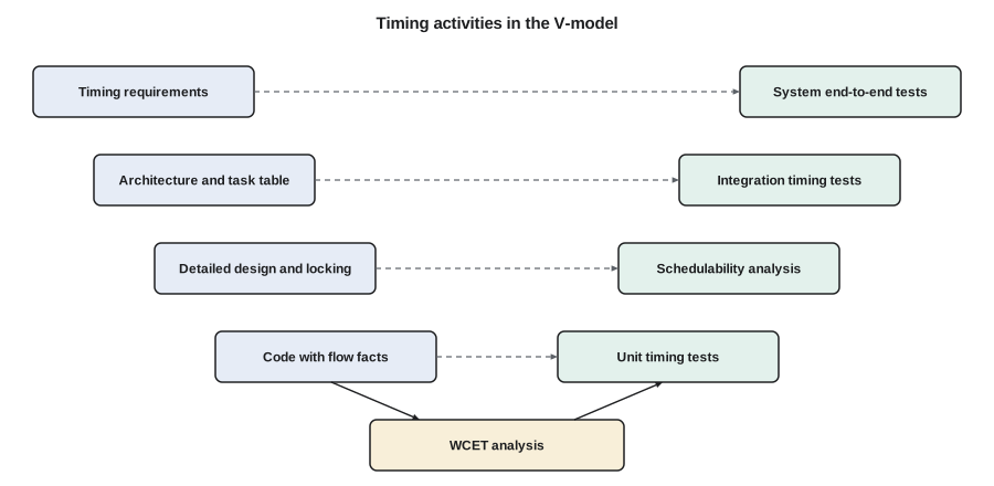
Traceability ties the two sides together. Each timing requirement should trace forward to the design elements that implement it and the verification results that show it is met, and each verification result should trace back to a requirement. When a requirement changes, traceability shows which analyses must be repeated; when an analysis fails, it shows which requirement is at risk.
Verification methods
Schedulability analysis, the subject of lessons 3 to 11, is the central timing verification method. It is only as valid as its inputs, so the analysis report must state its assumptions: the task model, the WCET values and how they were obtained, the overhead measurements, the blocking terms, the interrupt rates and any minimum interarrival times enforced by drivers. Reviewers check those assumptions as carefully as the arithmetic.
Timing tests run the system on target hardware and measure response times and end-to-end latencies. Tests cannot prove the worst case, as lesson 1 showed, but they validate the analysis: a measured response time above the computed bound means the model is wrong. Good timing tests stress the system deliberately, aligning releases to approximate the critical instant, saturating interrupts at their maximum rates, forcing the slow paths found by WCET analysis and loading the CAN bus with worst-case traffic. Trace tools that record every context switch, interrupt and kernel call with timestamps make the results interpretable; the trace that diagnosed the Mars Pathfinder inversion is the classic example.
Model checking explores every possible behavior of a model of the system. For real-time systems, models are often timed automata, finite-state machines extended with real-valued clocks and constraints on them, introduced by Alur and Dill in 1994. A model checker can verify properties such as 'the vehicle call is always sent within 2 ms of a confirmed detection' over all interleavings of the model. Model checking finds subtle errors in protocols and mode logic, such as the transition into HI mode in a mixed-criticality system, but the state space grows quickly with system size, so it is applied to critical parts rather than whole products.
Run-time monitoring keeps checking timing in the field. Deadline monitors record any job that finishes late; execution-time monitors enforce budgets and detect overruns; watchdogs detect tasks that stop running altogether. On the NS-5 the kernel's budget timers, the classifier's high-water mark and a watchdog supervised by the cyclic supervisor of lesson 3 provide three independent layers. Monitoring turns a violated assumption into a detected event with a defined response, rather than a silent failure.
Fault injection checks the responses: the team deliberately makes the classifier overrun, floods the CAN receive interrupt, corrupts frames on the bus and stops a task, and checks that each fault is detected and handled as the safety analysis expects.
Functional safety standards
Functional safety standards define how much rigor is needed according to how much risk a function controls. They share a common pattern: a hazard and risk analysis assigns each safety function an integrity level, and the level determines the required development process, the techniques that are highly recommended and the evidence that must be produced.
| Standard | Domain | Integrity levels | Notes |
|---|---|---|---|
| IEC 61508 | Generic electrical, electronic and programmable systems | SIL 1 to SIL 4 | The parent standard from which many sector standards are derived |
| ISO 26262 (2nd edition 2018) | Road vehicles | ASIL A to ASIL D | QM for functions with no safety requirement; ASIL decomposition across redundant elements |
| DO-178C (2011) | Airborne software | DAL A to DAL E | Objectives per level, with independence of verification at the higher levels |
| IEC 62304 | Medical device software | Classes A, B and C | Used with ISO 14971 risk management |
| EN 50128 and EN 50716 | Railway software | SIL 0 to SIL 4 | EN 50716 published in 2023 to supersede EN 50128 |
For timing, these standards expect worst-case execution times and schedulability to be analyzed, not merely tested, at the higher integrity levels. ISO 26262 lists freedom from interference as a requirement whenever elements of different ASIL share a processor: a lower-ASIL element must not be able to delay a higher-ASIL element beyond what the analysis allows. Timing protection through budgets, partitioning and deadline monitoring is the standard way to provide it, which connects directly to the mixed-criticality design of lesson 8. DO-178C and its supplements require evidence that worst-case execution time and stack usage have been determined for the actual target, and the multicore guidance discussed in lesson 9 adds interference analysis.
Coding standards support analyzability. MISRA C, first published in 1998 for the automotive industry and now used widely in safety-related embedded software, restricts the C language to a subset that avoids undefined and implementation-specific behavior and constructs that hamper analysis: it discourages dynamic memory allocation, unbounded recursion and certain uses of pointers and type conversion. Its rules overlap strongly with the design-for-analyzability advice of lesson 10. Static analyzers check conformance automatically, and deviations are documented and justified.
Safety cases
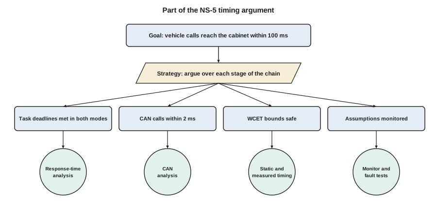
A safety case is a structured argument, supported by evidence, that a system is acceptably safe for a given application in a given environment. Timing evidence is one strand of it. Arguments are often drawn in goal structuring notation (GSN), in which a top-level claim such as 'vehicle calls are delivered in time' is broken into sub-claims, each supported by strategies and finally by evidence items such as analysis reports, test results and review records. Writing the argument explicitly exposes gaps: a claim supported only by testing at a level where the standard expects analysis, or an analysis whose WCET inputs came from measurements with no coverage argument.
Capstone: the NS-5 timing sign-off
Jonah's presentation brings together every lesson. The release configuration runs the base classifier, with C(LO) = 6 ms from measurement and C(HI) = 9 ms from static analysis with margin, the statistics task added for the city's traffic office, and a polling server, SERVICE, with a budget of 0.2 ms every 10 ms for the service port commands that Dev asked to speed up in lesson 8. RADAR, CANTX and CLASS are HI-criticality; SERVICE, STATS, LOG and HOUSE are LO-criticality and are suspended in HI mode. Priorities are rate-monotonic. Shared resources use the immediate ceiling protocol, giving the blocking terms of lesson 7. Kernel overheads come from lesson 6's measurements, and the CAN bus analysis from lesson 11. The pedestrian-detection feature, with its 11 ms classifier, does not fit on one core together with the statistics task, since the combined LO-mode utilization would exceed 1; it moves to the dual-core NS-5D, where lesson 9 showed a feasible partition.
The script below is the sign-off calculation. It performs AMC response-time analysis with context switches, the tick and interrupt handlers, and blocking included, and then computes the end-to-end latency using the HI-mode response times, which are the worst that can occur.
from math import ceil

# NS-5 release configuration, times in microseconds, rate-monotonic priority order
CS = 5                                                   # context switch, charged twice per job
ISRS = [("tick", 8, 1_000), ("radar DMA", 15, 6_250), ("CAN rx", 6, 188)]
TASKS = [  # name, criticality, C(LO), C(HI), T = D, blocking B
    ("RADAR", "HI", 1_200, 1_600, 6_250, 150), ("CANTX", "HI", 800, 1_000, 10_000, 150),
    ("SERVICE", "LO", 200, 200, 10_000, 0),
    ("STATS", "LO", 4_000, 4_000, 20_000, 0),  ("CLASS", "HI", 6_000, 9_000, 25_000, 0),
    ("LOG", "LO", 8_000, 8_000, 100_000, 300), ("HOUSE", "LO", 20_000, 20_000, 1_000_000, 0)]

def solve(base, terms, limit):
    r = base
    while True:
        nxt = base + sum(ceil(r / t) * c for c, t in terms)
        if nxt == r or nxt > limit:
            return nxt
        r = nxt

isr_terms = [(c, t) for _, c, t in ISRS]
report, results = [], {}
for i, (n, crit, clo, chi, t, b) in enumerate(TASKS):
    hp = TASKS[:i]
    lo_terms = isr_terms + [(x[2] + 2 * CS, x[4]) for x in hp]
    rlo = solve(clo + 2 * CS + b, lo_terms, t)
    rhi = None
    if crit == "HI":
        frozen = sum(ceil(rlo / x[4]) * (x[2] + 2 * CS) for x in hp if x[1] == "LO")
        hi_terms = isr_terms + [(x[3] + 2 * CS, x[4]) for x in hp if x[1] == "HI"]
        rhi = solve(chi + 2 * CS + b + frozen, hi_terms, t)
    ok = rlo <= t and (rhi is None or rhi <= t)
    results[n] = rhi if rhi is not None else rlo
    report.append((n, crit, rlo, rhi, t, ok))

print("task    crit  R_LO (ms)  R_HI (ms)  D (ms)")
for n, crit, rlo, rhi, t, ok in report:
    hi = f"{rhi/1000:9.2f}" if rhi is not None else "        -"
    print(f"{n:7s} {crit:4s}  {rlo/1000:9.2f}  {hi}  {t/1000:6g}  {'ok' if ok else 'MISS'}")

# end-to-end: vehicle enters beam -> cabinet controller uses the call (HI-mode values)
chain = [("wait for next radar frame", 6_250), ("RADAR response", results["RADAR"]),
         ("wait for next CLASS release", 25_000), ("CLASS response", results["CLASS"]),
         ("CAN vehicle call, node 4", 1_240), ("cabinet detector poll", 20_000)]
total = sum(v for _, v in chain)
print("\nend-to-end chain")
for name, v in chain:
    print(f"  {name:28s} {v/1000:6.2f} ms")
print(f"  {'total':28s} {total/1000:6.2f} ms   requirement 100 ms   margin {(100_000-total)/1000:.2f} ms")
print("all deadlines met:", all(r[5] for r in report) and total <= 100_000)task crit R_LO (ms) R_HI (ms) D (ms) RADAR HI 1.44 1.85 6.25 ok CANTX HI 2.29 2.90 10 ok SERVICE LO 2.35 - 10 ok STATS LO 7.80 - 20 ok CLASS HI 16.40 23.93 25 ok LOG LO 49.23 - 100 ok HOUSE LO 173.79 - 1000 ok end-to-end chain wait for next radar frame 6.25 ms RADAR response 1.85 ms wait for next CLASS release 25.00 ms CLASS response 23.93 ms CAN vehicle call, node 4 1.24 ms cabinet detector poll 20.00 ms total 78.27 ms requirement 100 ms margin 21.73 ms all deadlines met: True
Every task meets its deadline in LO mode, and every HI task meets its deadline in HI mode. The tightest result is the classifier in HI mode, 23.93 ms against 25 ms, a margin of 1.07 ms, or about 4 %. The service port server answers within 2.35 ms in LO mode. The end-to-end worst case is 78.27 ms against the 100 ms requirement, a margin of 21.73 ms.
The review raises three points. Ines asks whether a 4 % margin on the classifier in HI mode is enough. Jonah's answer is that HI mode is entered only when the classifier itself overruns its measured bound, and that the margin is on top of a static bound that already includes the rare slow path; still, he records a design rule that any change to the classifier's code must rerun the static timing analysis before release, and the sensitivity analysis shows that C(HI) can grow to about 10.0 ms before CLASS misses in HI mode. Dev asks whether the service port will slow the radar; it cannot, because service commands run in the SERVICE server below RADAR and CANTX with an enforced budget, and the analysis above already includes it. Dana asks what the city will see if HI mode is entered; statistics pause for at most one hyperperiod and the event is logged and reported in the next upload, which her server team will display as a data gap rather than a zero count.
The sign-off package the team submits contains the timing requirements with their sources; the task table and the CAN message table; the WCET reports, both static and measured; the overhead measurements; the schedulability and end-to-end analysis; the results of stress and fault-injection tests that validate the analysis; the run-time monitoring design; and the safety argument that links them. It is the deliverable this course has been building toward.
Worked problem
Finding the largest safe classifier bound
Using the sign-off model, Jonah wants the largest C(HI) for CLASS that keeps CLASS schedulable in HI mode. In HI mode, CLASS's response time is its own C(HI) plus context switches, frozen interference from the LO tasks STATS and SERVICE up to the LO-mode response time, the HI interference from RADAR and CANTX at their HI values and the interrupt load. At C(HI) = 9 ms the result is 23.93 ms. How can the limit be found?
Show solution
- Each additional millisecond of C(HI) adds at least 1 ms to R(HI) and may add further preemptions by RADAR, 1.61 ms each, and CANTX, 1.01 ms each, when R(HI) crosses one of their release times.
- The 1.07 ms margin cannot absorb an extra RADAR preemption on top of the added execution, so the limit lies below 9 + 1.07 = 10.07 ms.
- A binary search over C(HI) with the same analysis finds the largest value for which R(HI) ≤ 25 ms; this is the sensitivity analysis of lesson 4.
- The search gives a limit of 10.03 ms, which Jonah records as a design rule of 10.0 ms.
Answer: About 10.0 ms; any classifier change that pushes the static bound above that value needs a redesign.
Where to go next
This course has covered the core of real-time systems: task models, cyclic and priority-driven scheduling, response-time and demand analysis, operating system mechanisms, resource sharing, servers and mixed criticality, multicore scheduling, timing analysis and real-time networks. The research literature continues in every one of these directions, with active work on multicore interference, mixed-criticality certification, timing analysis for machine-learning workloads and real-time guarantees in large distributed and cloud systems. The engineering habit at the center of it all is the one introduced in lesson 1: state timing requirements precisely, reason about the worst case rather than the average, and keep the evidence that the worst case is covered.
Common mistakes
MistakePresenting analysis results without their assumptions.
InsteadState the model, WCET sources, overheads, blocking and enforced interarrival times with every result.
MistakeTreating timing tests as proof of the worst case.
InsteadUse tests to validate analysis; a measured value above a bound means the model is wrong.
MistakeLetting lower-criticality functions share a processor without timing protection.
InsteadProvide freedom from interference with budgets, partitions and deadline monitoring.
MistakeSigning off with no margin policy.
InsteadRecord margins and the design rules that keep them, such as rerunning WCET analysis after code changes.
MistakeWriting the safety case after the design is finished.
InsteadBuild the argument alongside the design so gaps in evidence show up early.
Summary and key terms
- Timing verification spans the whole V-model, from requirements with sources to end-to-end system tests.
- Schedulability analysis is central but valid only with stated, checked assumptions.
- Timing tests, tracing, model checking, run-time monitoring and fault injection complement analysis.
- IEC 61508, ISO 26262, DO-178C, IEC 62304 and railway standards set integrity levels that determine rigor.
- Freedom from interference and analyzable code, for example under MISRA C, support timing arguments.
- A safety case links timing claims to evidence in a structured argument.
- The NS-5 sign-off meets every deadline in both modes with an end-to-end worst case of 78.27 ms.
- V-model
- A development model that pairs each design level with a corresponding verification level.
- Traceability
- Links between requirements, design elements and verification results.
- Timed automaton
- A finite-state machine extended with real-valued clocks, used for model checking timing properties.
- Safety integrity level
- A level that sets the rigor required for a safety function, such as SIL, ASIL or DAL.
- Freedom from interference
- Assurance that one element cannot cause another of higher criticality to fail.
- MISRA C
- A widely used set of rules restricting C for safety-related embedded software.
- Safety case
- A structured argument, supported by evidence, that a system is acceptably safe in its context.
- Goal structuring notation (GSN)
- A graphical notation for safety arguments built from goals, strategies and evidence.
Practice problems
Work each problem on paper first, then reveal the answer to check.
Which integrity level is the most demanding in ISO 26262, and which in DO-178C?
Show answer
ASIL D and DAL A.
A measured response time of CLASS is 24.3 ms, but analysis gives 23.93 ms in HI mode. What does this mean?
Show answer
The analysis model is wrong somewhere; find the missing interference, overhead or execution-time effect before trusting any result.
Why does the pedestrian feature move to the NS-5D?
Show answer
With the 11 ms classifier and the statistics task, LO-mode utilization exceeds 1 on one core.
What three independent run-time timing protections does the NS-5 use?
Show answer
Kernel budget timers, the classifier high-water mark with mode switch, and a watchdog supervised by the cyclic supervisor.
Lesson quiz · 5 questions
Score 60% or more to complete this lesson.
Create a free account to save your progress, take quizzes and earn a certificate.