
CMP-440 · Lesson 11 of 12 · 21 min
Real-time communication: CAN and time-sensitive networking
Most real-time functions span more than one computer. A vehicle call from the NS-5 is useful only when it reaches the signal controller in the cabinet; a brake command matters only when it reaches the wheel actuators; a sensor reading in a factory is useful only when the controller has it. The network between them is therefore part of the real-time system, and its delays must be bounded just as carefully as task response times. This lesson shows how the controller area network (CAN), the dominant real-time bus in vehicles and industrial equipment, can be analyzed with the same response-time methods as tasks, and how time-sensitive networking (TSN) brings bounded latency to Ethernet. It ends with end-to-end analysis across tasks and networks, completing the calculation begun in lesson 1.
In the cabinet, the NS-5 nodes on each approach share a CAN bus at 500 kbit/s with the signal controller. Lesson 1 gave the vehicle-call message a 2 ms deadline from queuing to reception. With four NS-5 nodes on a typical Ann Arbor intersection and the controller's own traffic, Jonah must show that every vehicle call meets that deadline in the worst case.
CAN as a fixed-priority scheduler
CAN, introduced in the 1980s and standardized as ISO 11898, is a multi-master serial bus in which any node may begin transmitting when the bus is idle. CMP-315 described its bitwise arbitration: each frame begins with an identifier, a dominant 0 bit overwrites a recessive 1 on the wire, and a node that sends a recessive bit but reads a dominant one has lost and stops transmitting. The frame with the numerically lowest identifier therefore always wins, without destroying anyone's transmission. From a scheduling point of view, CAN is a fixed-priority, non-preemptive scheduler whose priorities are the identifiers. Once a frame has started, it runs to completion even if a higher-priority frame becomes ready.
That observation, made by Tindell, Burns and Wellings in 1994, lets CAN messages be analyzed like tasks. Each message stream m has a transmission time C_m, a period or minimum interarrival time T_m, a deadline D_m and a queuing jitter J_m, the variation in the time from the event to the frame being placed in the controller's transmit buffer, which comes from the response time of the sending task. Because transmission is non-preemptive, a message can be blocked by one lower-priority frame that started just before it was queued: the blocking term B_m is the longest transmission time among lower-priority messages.
Frame transmission times
A CAN frame's length depends on the number of data bytes and on bit stuffing: after five consecutive bits of the same value, the transmitter inserts a complementary bit, so a frame's length on the wire depends on its content. The worst case for a standard 11-bit identifier frame with s data bytes, including the 3-bit interframe space, is:
Here 47 bits are the fixed fields and interframe space, 8s are the data bits, and the floor term is the worst-case number of stuff bits over the 34 + 8s bits subject to stuffing. At 500 kbit/s, τ_bit = 2 µs, so an 8-byte frame takes up to 135 bits or 270 µs, the value used in CMP-315, and a 2-byte vehicle call up to 75 bits or 150 µs.
Response-time analysis for CAN
The queuing delay w_m of message m, the time from being queued to starting transmission successfully, satisfies an equation like the task equation of lesson 4, with the blocking term and with jitter on the interfering messages. The extra τ_bit appears because a higher-priority message queued up to one bit time after m's transmission has started arbitration can still win:
The original analysis contained a subtle flaw. In 2007 Davis, Burns, Bril and Lukkien showed that it could be optimistic for messages at high load, because the transmission of one instance of a message can delay the next instance of the same message when their combined busy period extends past the period, and a message set that the original test accepted could miss deadlines in practice. Their revised analysis examines every instance in the busy period. They also gave a simple sufficient form that is safe for any message set: replace B_m with the larger of B_m and C_m. The code below uses that form for the cabinet bus.
The bus carries the controller's signal-phase broadcast with identifier 0x080, an 8-byte frame every 10 ms; a 2-byte vehicle call from each of four nodes, identifiers 0x101 to 0x104, with minimum separation 10 ms, deadline 2 ms and queuing jitter 100 µs from the sending task; an 8-byte status frame from each node every 25 ms; an hourly count report sent in pieces at most once a second; and a diagnostics frame every 50 ms at the lowest priority, identifier 0x700.
from math import ceil

BIT = 2.0                       # microseconds per bit at 500 kbit/s

def frame_bits(data_bytes):
    """worst-case length of a standard-identifier CAN frame including stuff bits and the interframe space"""
    s = data_bytes
    return 47 + 8 * s + (34 + 8 * s - 1) // 4

# (name, identifier, data bytes, period or minimum interarrival T, deadline D, queuing jitter J), times in us
msgs = [("signal phase", 0x080, 8, 10_000, 10_000, 0),
        ("call node 1", 0x101, 2, 10_000, 2_000, 100), ("call node 2", 0x102, 2, 10_000, 2_000, 100),
        ("call node 3", 0x103, 2, 10_000, 2_000, 100), ("call node 4", 0x104, 2, 10_000, 2_000, 100),
        ("status node 1", 0x200, 8, 25_000, 25_000, 500), ("status node 2", 0x201, 8, 25_000, 25_000, 500),
        ("status node 3", 0x202, 8, 25_000, 25_000, 500), ("status node 4", 0x203, 8, 25_000, 25_000, 500),
        ("counts", 0x300, 8, 1_000_000, 1_000_000, 1_000), ("diagnostics", 0x700, 8, 50_000, 50_000, 0)]
msgs.sort(key=lambda m: m[1])                    # lower identifier wins arbitration
C = {m[0]: frame_bits(m[2]) * BIT for m in msgs}

print(f"8-byte frame {frame_bits(8)} bits = {frame_bits(8)*BIT:.0f} us, 2-byte frame {frame_bits(2)} bits = {frame_bits(2)*BIT:.0f} us")
print(f"bus utilization {sum(C[m[0]] / m[3] for m in msgs):.3f}")
print("message         id     C(us)  B(us)   R(us)    D(us)")
for i, (name, ident, n, T, D, J) in enumerate(msgs):
    lower = [C[m[0]] for m in msgs[i + 1:]]
    B = max(lower + [C[name]])                   # Davis et al. simple sufficient form: max(B, C)
    w = B
    while True:
        nxt = B + sum(ceil((w + Jk + BIT) / Tk) * C[k] for k, _, _, Tk, _, Jk in msgs[:i])
        if nxt == w or nxt + C[name] + J > D:
            break
        w = nxt
    R = J + nxt + C[name]
print(f"{name:14s} 0x{ident:03X} {C[name]:5.0f} {B:5.0f} {R:7.0f} {D:7d} {'met' if R <= D else 'MISSED'}")8-byte frame 135 bits = 270 us, 2-byte frame 75 bits = 150 us bus utilization 0.136 message id C(us) B(us) R(us) D(us) signal phase 0x080 270 270 540 10000 met call node 1 0x101 150 270 790 2000 met call node 2 0x102 150 270 940 2000 met call node 3 0x103 150 270 1090 2000 met call node 4 0x104 150 270 1240 2000 met status node 1 0x200 270 270 1910 25000 met status node 2 0x201 270 270 2180 25000 met status node 3 0x202 270 270 2450 25000 met status node 4 0x203 270 270 2720 25000 met counts 0x300 270 270 3490 1000000 met diagnostics 0x700 270 270 2760 50000 met
The bus utilization is only 0.136, but utilization says little about worst-case latency on a non-preemptive bus. The signal phase broadcast can be delayed by one diagnostics frame already on the wire, so its response time is 540 µs. Each vehicle call waits for one blocking frame, the signal phase broadcast and every higher-priority call: node 1's call is received within 790 µs and node 4's within 1,240 µs, both within the 2 ms deadline, with 760 µs of margin for node 4. If identifiers were assigned carelessly, with the vehicle calls above 0x300, they could be delayed behind the status frames as well; identifier assignment on CAN is priority assignment, and deadline-monotonic ordering is as sensible here as on a processor.
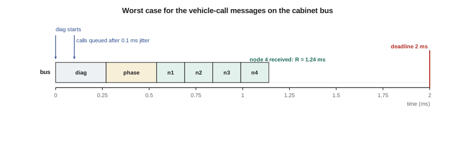
Two further effects belong in a complete analysis. Errors cause retransmissions: a frame corrupted by noise is destroyed by an error frame and retransmitted, adding the error frame and the retransmitted frame to the response time of every message that waits behind it. Analyses add an error term based on an assumed maximum error rate, such as one error every 10 ms in a noisy environment. And CAN controllers must be configured so that the hardware transmit buffers do not cause priority inversion: a controller with a single first-in, first-out transmit buffer can hold a low-priority frame at the head while a high-priority frame waits behind it, breaking the analysis. The NS-5's controller has three prioritized transmit buffers and sends the lowest identifier first, which preserves the analysis.
Beyond classical CAN
Classical CAN carries at most 8 data bytes at up to 1 Mbit/s. CAN FD, standardized in ISO 11898-1 in 2015, keeps arbitration at the classical rate but switches to a faster bit rate, commonly 2 to 5 Mbit/s, for the data phase, and allows up to 64 data bytes. CAN XL extends payloads to 2,048 bytes and data rates to 10 Mbit/s or more. The same response-time analysis applies with the new frame-length formulas, since arbitration remains fixed-priority and non-preemptive. Other fieldbuses take different approaches: FlexRay combines a time-triggered static segment with an event-driven dynamic segment, and many industrial Ethernet protocols use a master that polls slaves on a fixed cycle.
Time-sensitive networking
Ethernet offers far more bandwidth than CAN, but standard switched Ethernet gives no latency guarantee: frames queue behind other traffic in switch output buffers for as long as the traffic pattern dictates. Time-sensitive networking is a family of IEEE 802.1 standards that add bounded latency, low jitter and high reliability to Ethernet, so that control traffic and ordinary traffic can share one network. The main pieces are these.
| Standard | Function |
|---|---|
| IEEE 802.1AS | Precise time synchronization across all switches and end stations, a profile of the Precision Time Protocol, typically to well under 1 µs |
| IEEE 802.1Qbv | Time-aware shaper: each output port opens and closes the gate of each traffic class according to a repeating gate control list on synchronized time |
| IEEE 802.1Qav | Credit-based shaper: limits the rate of audio and video streams to smooth bursts and bound latency for other classes |
| IEEE 802.1Qbu and IEEE 802.3br | Frame preemption: an express frame can interrupt a long frame in progress, which resumes afterwards |
| IEEE 802.1CB | Frame replication and elimination: frames are sent over disjoint paths and duplicates are removed, tolerating link or switch failures |
| IEEE 802.1Qcc | Stream reservation and configuration of the network for time-sensitive streams |
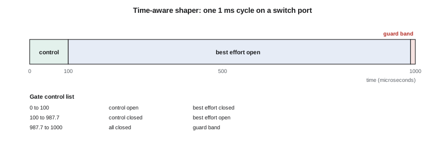
The time-aware shaper is the most direct counterpart of the cyclic executive in lesson 3. A network-wide schedule repeats every cycle, for example 1 ms. In each cycle, every switch port opens a window during which only the scheduled traffic class may transmit, and closes it for everyone else. If the schedules of successive switches are aligned with the expected arrival times, a scheduled frame travels the network with almost no queuing, and its latency is close to the sum of its transmission and propagation times. A guard band before each protected window, long enough for the longest other frame, ensures that no frame is still being transmitted when the window opens; frame preemption shrinks the guard band from a full-size frame to a fragment.
Worked problem
Sizing a guard band
A 1 Gbit/s TSN port carries best-effort frames of up to 1,522 bytes, plus an 8-byte preamble and a 12-byte interframe gap. How long must the guard band before a protected window be, with and without frame preemption, if a preemptable fragment can be at most 143 bytes on the wire?
Show solution
- \[ t_{\text{max frame}} = \frac{(1522 + 8 + 12) \times 8}{10^9} = 12.336\ \mu\text{s}\]
- Without preemption the guard band must cover a whole maximum frame, 12.336 µs, wasting up to 1.2 % of a 1 ms cycle.
- \[ t_{\text{fragment}} = \frac{143 \times 8}{10^9} = 1.144\ \mu\text{s}\]
- With preemption, the guard band only has to cover the largest non-preemptable fragment.
Answer: 12.336 µs without preemption and 1.144 µs with it.
Northway Sensing is evaluating TSN for a future cabinet backbone that would connect radar nodes, cameras and the signal controller on one Ethernet network. For the NS-5 generation, CAN remains: it is cheap, robust in electrically noisy cabinets, and, as the analysis shows, its latency is easily bounded for this traffic.
End-to-end timing
With task response times from lessons 4 to 7 and message response times from this lesson, the end-to-end calculation of lesson 1 can be redone with real numbers. The holistic analysis of Tindell and Clark, published in 1994, formalizes this: the response time of each task in a chain becomes release jitter for the message it sends, and the message's response time becomes release jitter for the task that receives it, iterating until every value is stable. For the NS-5 chain, the event-triggered design gives a worst case of: up to 6.25 ms for the vehicle to appear in a frame, 1.35 ms for RADAR including blocking, up to 25 ms of sampling wait plus 16.99 ms for CLASS with the heavy classifier and overheads, 1.24 ms for the vehicle call on the bus, and up to 20 ms for the cabinet's detector poll. The total is 70.83 ms against the 100 ms requirement, and every number in the sum is now backed by analysis rather than by a deadline used as a placeholder.
Common mistakes
MistakeUsing bus utilization to judge CAN latency.
InsteadRun response-time analysis; non-preemptive blocking and priorities dominate latency.
MistakeUsing the original CAN analysis at high load.
InsteadUse the 2007 revised analysis or its sufficient form with max(B_m, C_m).
MistakeAssigning CAN identifiers without regard to deadlines.
InsteadIdentifiers are priorities; assign them deadline-monotonically.
MistakeUsing a controller with a single FIFO transmit buffer for mixed-priority traffic.
InsteadUse prioritized transmit buffers so local priority inversion cannot occur.
MistakeAdding network latency to task latency without accounting for jitter.
InsteadUse holistic analysis so each stage's response time becomes the next stage's jitter.
Summary and key terms
- CAN arbitration makes the bus a fixed-priority, non-preemptive scheduler with identifiers as priorities.
- An 8-byte standard frame is up to 135 bits, 270 µs at 500 kbit/s; a 2-byte frame is up to 75 bits.
- CAN response time is jitter plus queuing delay plus transmission time, with one lower-priority frame of blocking.
- The 2007 revised analysis corrected an optimistic flaw; max(B_m, C_m) gives a simple safe form.
- The NS-5 vehicle calls are received within 1.24 ms in the worst case, inside their 2 ms deadline.
- TSN adds time synchronization, gated scheduling, shaping, preemption and redundancy to Ethernet.
- Holistic analysis chains task and message response times into an end-to-end bound.
- Controller area network (CAN)
- A multi-master serial bus with bitwise priority arbitration.
- Bit stuffing
- Insertion of a complementary bit after five identical bits, which lengthens frames.
- Queuing jitter
- Variation in the time at which a message is placed in the transmit buffer.
- Time-sensitive networking (TSN)
- IEEE 802.1 standards that add bounded latency and reliability to Ethernet.
- Time-aware shaper
- A switch mechanism that opens and closes traffic-class gates on a synchronized schedule.
- Guard band
- A closed interval before a protected window that keeps other frames off the link.
- Frame preemption
- Interrupting a long frame to send an express frame, then resuming it.
- Holistic analysis
- End-to-end analysis that passes response times between tasks and messages as jitter.
Practice problems
Work each problem on paper first, then reveal the answer to check.
What is the worst-case length of a 4-byte standard CAN frame?
Show answer
47 + 32 + floor(65/4) = 79 + 16 = 95 bits, 190 µs at 500 kbit/s.
If the diagnostics frame were raised to identifier 0x050, what would happen to node 1's call?
Show answer
It would gain another higher-priority 270 µs frame of interference, so its response time would rise by about 270 µs.
Why does a TSN guard band need frame preemption to be short?
Show answer
Without preemption it must cover a whole maximum-length frame.
In the end-to-end sum, which single stage contributes most?
Show answer
The 25 ms sampling wait for the classifier.
Lesson quiz · 5 questions
Score 60% or more to complete this lesson.
Create a free account to save your progress, take quizzes and earn a certificate.