
CMP-440 · Lesson 1 of 12 · 21 min
What makes a system real-time
Most software is judged on whether it produces the right answer. A real-time system is judged on whether it produces the right answer at the right time. An airbag controller that decides correctly to fire, but 80 ms after the crash instead of 15 ms, has failed as completely as one that never fires. A pacemaker that paces correctly but a few hundred milliseconds late can stop a heart. A video player that drops one frame in a thousand is merely annoying. All three are real-time systems, and the differences between them are the subject of this lesson: what a deadline is, what happens when one is missed, which timing constraints a design must state, and why real-time engineering is about predictability rather than raw speed.
This course follows Northway Sensing, the Ann Arbor, Michigan company whose roadside traffic counters you met in CMP-200 through CMP-350. Its new product, the NS-5, does more than count. It classifies each vehicle from radar returns on the node itself, at 160 radar frames per second, and reports detections over a CAN bus to the traffic signal controller in the roadside cabinet, which uses them to extend a green phase or call a turning arrow. That last job changes everything. A count that arrives a minute late is still a correct count; a vehicle call that arrives after the signal has turned red is worthless, and in the worst case it leaves a driver waiting at an empty intersection or misses a cyclist entirely. Firmware lead Maren Holt has asked Jonah Abara, now on his final co-op term, to own the NS-5's timing analysis.
Correct in value and correct in time
The classic definition is that a real-time system is one whose correctness depends not only on the logical result of a computation but also on the time at which the result is produced. Every output therefore has two parts to check: the value and the instant. The instant is usually expressed as a deadline, the latest time by which a result must be produced, measured from some triggering event called the release. Some systems also have earliest times: a fuel injector must not fire before the right crank angle, and a sample must not be taken before the anti-aliasing filter settles. Real-time requirements are therefore windows, not just upper limits.
Real-time does not mean fast. A system that must respond within 2 s to a fire alarm is real-time; a supercomputer that renders a film overnight is not, however fast it is. What makes a system real-time is that it has stated timing constraints and that it must be shown to meet them, not merely on average but in the worst case that can occur. That shift from average to worst case is the core idea of the whole discipline. A desktop operating system is designed to make the common case fast and to share the processor fairly; a real-time system is designed to make the worst case bounded and known, even if that makes the average case slower.
Hard, firm and soft deadlines
Deadlines differ in what a miss costs. Engineers usually sort them into three classes, described by a utility function: the value to the system of a result as a function of the time it is produced.
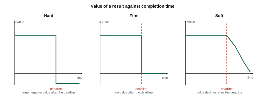
A hard deadline is one where a miss may cause a catastrophic failure: injury, death, destruction of equipment or serious financial or environmental harm. Flight control surfaces, airbag deployment, anti-lock braking, medical infusion pumps and the interlocks on a press brake have hard deadlines. A hard real-time system must be shown, by analysis rather than by testing alone, never to miss them under the assumptions it was designed for.
A firm deadline is one where a late result has no value but causes no harm beyond the loss of that result. A radar frame that is processed after the next frame has overwritten its buffer is simply discarded; a stock quote that arrives after the trade has closed is worthless. Firm systems can tolerate occasional misses if they are rare and bounded, and are often specified with statements such as 'no more than one miss in any ten consecutive frames'.
A soft deadline is one where a late result still has some value, which decreases with lateness. Video and audio playback, user interface response and most web services have soft deadlines. Soft real-time systems are evaluated statistically: the 99th percentile latency, the fraction of frames delivered on time, the mean tardiness. Many products contain all three classes. The NS-5 has a hard-in-practice deadline on reporting a vehicle call to the cabinet, because signal timing depends on it, a firm deadline on each radar frame and soft deadlines on uploading counts to the server and refreshing its service display.
| System | Event | Typical deadline | Class |
|---|---|---|---|
| Airbag controller | Crash detected | About 15 to 30 ms to fire | Hard |
| Anti-lock braking | Wheel slip measured | A few ms per control cycle | Hard |
| Pacemaker | Missed natural beat | Tens of ms | Hard |
| NS-5 vehicle call | Vehicle enters detection zone | 100 ms to reach the cabinet | Hard in practice |
| NS-5 radar frame | Frame buffer full | 6.25 ms, before the next frame overwrites it | Firm |
| Video playback | Frame due | 16.7 ms at 60 frames per second | Soft |
| NS-5 count upload | Hourly report due | Minutes | Soft |
Timing constraints a design must state
A requirement such as 'the system shall respond quickly' cannot be analyzed. A real-time specification states timing constraints precisely enough that each one can be checked. The most common are these.
Deadline: the maximum time from a release to completion. It may be relative, such as 10 ms after the sensor interrupt, or absolute, such as before 08:00:00.000. Period: for activities that repeat, the interval between releases, such as a control loop every 5 ms. Latency: the delay from an event to the start of the response, as in the interrupt latency of CMP-315. Jitter: the variation in timing from one instance to the next. Output jitter on a control loop, where the actuator is updated at slightly different points in each period, degrades control performance even if every deadline is met, because the controller's design assumed a constant sampling interval. Throughput: the rate at which work must be completed, such as 160 frames per second. End-to-end deadline: the limit on a chain of activities from a physical input to a physical output, which usually spans several tasks, a network and another computer.
Constraints also have sources, and each should be traceable to one. The NS-5's 100 ms limit on reporting a vehicle comes from the signal controller's detector input specification, which treats a call as valid for timing decisions only if it is fresh. The 6.25 ms frame deadline comes from the radar's double buffer: the DMA controller fills one half while the processor works on the other, so each half must be processed before DMA comes back to it. Writing these sources down matters, because when a deadline later proves hard to meet the first question is whether it can be relaxed, and only the source can answer that.
Time-triggered and event-triggered designs
Real-time systems take two broad approaches to deciding when to do things. In a time-triggered design, all activities start at predetermined instants derived from a global clock: read the sensors at 0 ms, compute at 1 ms, write the actuators at 4 ms, repeat every 5 ms. Behavior is fixed in advance, easy to analyze and test, and naturally free of jitter, but the system responds to an external event only at the next scheduled instant and wastes capacity when nothing happens. In an event-triggered design, activities start when events occur: an interrupt, a message, a timer expiry. Response can be immediate and idle time is used efficiently, but the timing depends on the pattern of events, which is harder to bound. Lesson 3 covers time-triggered cyclic executives; most of the rest of the course covers priority-driven, event-triggered scheduling with a real-time operating system. Real products usually mix the two: the NS-5 processes radar frames on a strict period set by the radar's own clock, but sends a vehicle call the moment classification confirms one.
Predictability is the goal
Because guarantees depend on the worst case, a real-time designer prefers mechanisms whose worst case is known, even at some cost to the average case. Caches, branch predictors, dynamic memory allocation, garbage collection, virtual memory paging and general-purpose schedulers all improve average performance while making the worst case hard to bound. A real-time system either avoids them, configures them for determinism, or accounts for their worst-case effects explicitly. The NS-5 locks its classification code and data into tightly coupled memory, allocates every buffer statically at startup and uses a real-time kernel whose every service has a bounded execution time. CMP-310 discussed caches and pipelines from the performance side; this course looks at them from the predictability side in lesson 10.
Worked problem
Does the first NS-5 design meet its end-to-end deadline?
Jonah traces the worst case from a vehicle entering the radar beam to the cabinet controller using the call. The vehicle can enter just after a frame starts, so it is seen only in the next frame: up to 6.25 ms. That frame is processed within its 6.25 ms deadline. Classification needs four frames of evidence, a 25 ms window, and the classifier task runs every 25 ms with a 25 ms deadline. In the first design, detections are queued and sent in a CAN message every 10 ms, with a 10 ms deadline. Finally, the signal controller reads its detector inputs every 20 ms. Is the 100 ms limit met in the worst case?
Show solution
- \[ R_{\text{e2e}} = 6.25 + 6.25 + 25 + 25 + 10 + 10 + 20\]
- \[ R_{\text{e2e}} = 102.5\ \text{ms}\]
- The worst case exceeds 100 ms by 2.5 ms, even though the typical latency, with every stage at about half its worst case, is about 51 ms.
- Sending the CAN message as soon as the classifier confirms a vehicle, with a 2 ms deadline, removes the 10 ms periodic wait and replaces the 10 ms response with 2 ms.
Answer: The first design does not guarantee the deadline; the event-triggered CAN message brings the worst case to 84.5 ms, a margin of 15.5 ms.
The example shows why worst-case reasoning matters. Bench tests of the first design, run for an afternoon with vehicles passing at random, never measured a latency above 70 ms. The 102.5 ms case requires every stage to hit its worst phasing at once, which is rare but certain to happen eventually over millions of vehicles a year across hundreds of intersections. The code below repeats the calculation for both designs and also estimates how often the bad alignment would occur if stage delays were independent and uniformly distributed.
import random
random.seed(440)

# worst-case delay of each stage in microseconds: (name, sampling wait, response bound)
first  = [("radar frame", 6_250, 6_250), ("classifier", 25_000, 25_000),
          ("CAN message", 10_000, 10_000), ("cabinet poll", 20_000, 0)]
second = [("radar frame", 6_250, 6_250), ("classifier", 25_000, 25_000),
          ("CAN message", 0, 2_000), ("cabinet poll", 20_000, 0)]

def worst(chain):
    return sum(w + r for _, w, r in chain)

def simulate(chain, n=200_000, limit=100_000):
    over = 0
    for _ in range(n):
        total = sum(random.uniform(0, w) + random.uniform(0.3 * r, r) for _, w, r in chain)
        over += total > limit
    return over / n

for name, chain in (("first design", first), ("event-triggered CAN", second)):
    print(f"{name:20s} worst case {worst(chain)/1000:6.2f} ms   "
f"fraction of random trials over 100 ms: {simulate(chain):.5f}")first design worst case 102.50 ms fraction of random trials over 100 ms: 0.00000 event-triggered CAN worst case 84.50 ms fraction of random trials over 100 ms: 0.00000
In 200,000 random trials the first design never exceeded 100 ms, not even once, because the violation needs every stage to sit close to its own worst case at the same moment. Random testing of this size would pass the design. Yet the analysis proves the violation exists. The event-triggered design can never exceed 100 ms. That contrast, between what testing samples and what analysis bounds, is the reason the rest of this course develops analytical tools: task models, schedulability tests, response-time analysis, blocking analysis and timing measurement.
Where real-time systems are found
Real-time requirements appear wherever computers interact with the physical world. Vehicles contain dozens of real-time controllers for engines, brakes, steering, batteries and driver assistance, connected by CAN and automotive Ethernet. Aircraft run flight control, engine control and avionics with hard deadlines under strict certification, discussed in lesson 12. Industrial plants use programmable logic controllers and motion controllers with cycle times from a few milliseconds down to tens of microseconds. Power grids rely on protection relays that must trip within a few cycles of the line frequency. Medical devices such as infusion pumps, ventilators and pacemakers have hard deadlines and regulated software processes. Telecommunications equipment processes radio frames on microsecond schedules. Even consumer products, such as earbuds with active noise cancellation, contain hard real-time signal paths.
Common mistakes
MistakeEquating real-time with fast.
InsteadReal-time means meeting stated timing constraints in the worst case; a slow system with a guaranteed bound can be real-time and a fast one without a bound is not.
MistakeValidating timing only by testing.
InsteadTesting samples typical cases; rare worst-case alignments need analysis to bound them.
MistakeSpecifying only deadlines.
InsteadState periods, jitter limits, latency and end-to-end constraints too, each traceable to its source.
MistakeTreating all deadlines as the same kind.
InsteadClassify each as hard, firm or soft and design the guarantees and tests to match.
MistakeUsing average-case mechanisms without accounting for their worst case.
InsteadCaches, dynamic allocation and general-purpose schedulers need determinism or explicit worst-case bounds.
Summary and key terms
- A real-time system is correct only if its results are right in value and in time.
- Real-time is about guaranteed worst-case timing, not about speed.
- Hard deadlines risk catastrophe, firm deadlines make late results useless, soft deadlines make them less valuable.
- Specifications state deadlines, periods, latency, jitter, throughput and end-to-end constraints, each with a source.
- Time-triggered designs act at fixed instants; event-triggered designs act on events; products often combine them.
- Predictable mechanisms with known worst cases are preferred over faster but unpredictable ones.
- Testing rarely finds worst-case alignments; analysis bounds them.
- Real-time system
- A system whose correctness depends on the time at which results are produced as well as on their values.
- Deadline
- The latest time by which a result must be produced, measured from its release.
- Release
- The instant at which an activity becomes ready to run.
- Hard deadline
- A deadline whose miss may cause catastrophic failure.
- Firm deadline
- A deadline after which a result has no value but causes no further harm.
- Soft deadline
- A deadline after which a result loses value gradually.
- Jitter
- Variation in the timing of a repeated activity from one instance to the next.
- End-to-end deadline
- A timing limit on a chain of activities from a physical input to a physical output.
Practice problems
Work each problem on paper first, then reveal the answer to check.
A control loop runs every 4 ms and the actuator is written between 1.1 ms and 1.9 ms after each release. What is the output jitter?
Show answer
1.9 − 1.1 = 0.8 ms.
Classify the deadline: a weather station must log a reading every 10 minutes, and a late reading is still stored with its true timestamp.
Show answer
Soft: a late reading keeps most of its value.
In the NS-5 example, by how much would the margin grow if the cabinet polled every 10 ms instead of 20 ms, with the event-triggered CAN message?
Show answer
The worst case falls from 84.5 to 74.5 ms, so the margin grows by 10 ms to 25.5 ms.
Why does a double-buffered DMA scheme give each buffer a deadline equal to the period?
Show answer
DMA returns to the same half one period later; processing must finish before it starts overwriting.
Lesson quiz · 5 questions
Score 60% or more to complete this lesson.
Create a free account to save your progress, take quizzes and earn a certificate.