Analog input and output: ADC, DAC and PWM

The physical world is analog. Battery voltage, temperature, light, pressure, current and sound vary continuously, and a microcontroller can only process numbers. The analog-to-digital converter turns a voltage into a number, the digital-to-analog converter turns a number back into a voltage, and pulse-width modulation fakes an analog output with a fast digital square wave and a filter. These three blocks connect firmware to every sensor and actuator that is not simply on or off. This lesson covers how they work, how to choose and configure them, and how to get trustworthy numbers out of real signals, which involves sampling theory, reference voltages, source impedance and a little filtering.

The NS-4 measures its battery voltage through the 100 kΩ and 27 kΩ divider that CMP-240 designed, and its solar charging current through a 50 mΩ sense resistor and an amplifier with a gain of 33. It reads an analog temperature sensor on the radar module, and it dims its status LED with PWM so that a technician at night is not dazzled. The NS-5 adds a DAC that sets the radar module's transmit power. All of these run through the microcontroller's analog peripherals.

Sampling and quantization

Converting a continuous signal to numbers involves two separate approximations. Sampling takes values only at discrete instants, typically evenly spaced at a sample rate f_s. Quantization rounds each value to one of a finite number of levels. An N-bit converter divides its input range, from 0 to the reference voltage V_ref, into 2ᴺ steps. The size of one step, one least significant bit, is the converter's resolution in volts. A 12-bit converter with a 3.3 V reference has 4,096 codes and an LSB of about 0.81 mV.

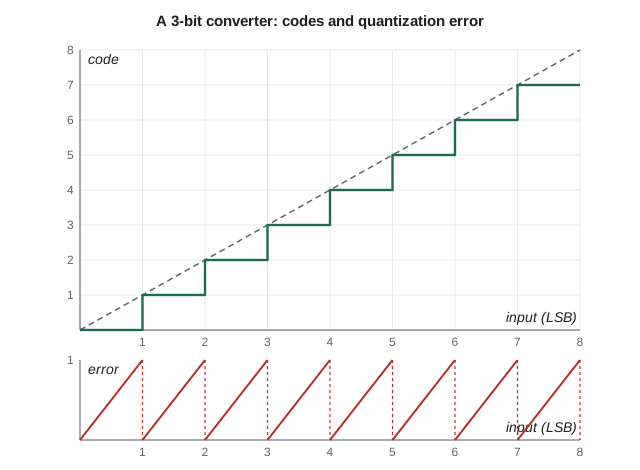
Quantization adds an error that, for a busy signal, behaves like random noise uniformly spread over one LSB. Its root-mean-square value is LSB divided by the square root of 12, and the resulting ideal signal-to-noise ratio for a full-scale sine wave is about 6.02N + 1.76 dB: 74 dB for 12 bits, 98 dB for 16 bits. Real converters fall short of this because of their own noise, nonlinearity and errors in the reference, so datasheets quote an effective number of bits, ENOB, which is often one to two bits below the nominal resolution. Resolution is how finely the converter divides its range; accuracy is how close the result is to the truth, and it is limited mostly by the reference voltage and by offset and gain errors, not by the number of bits.

How microcontroller ADCs work

Most microcontroller ADCs are successive-approximation converters. A sample-and-hold capacitor connects to the input for a programmable acquisition time, charging to the input voltage, and then disconnects. The converter then performs a binary search: it compares the held voltage with the output of an internal DAC set to half scale, keeps or clears the top bit depending on the result, sets the next bit, compares again, and continues for N steps. A 12-bit conversion needs 12 comparisons plus the acquisition time, typically 1 µs or less in total, giving sample rates up to about a million samples per second. A multiplexer in front of the converter selects one of many input pins, so one ADC serves many channels in turn, usually sequenced by hardware and fed to memory by DMA.

The acquisition time is where many measurements go wrong. The sample capacitor, typically 5 to 15 pF, must charge through the source impedance of whatever drives the pin. If the source is a high-value divider, the capacitor does not finish charging and the reading is low and depends on the previous channel. CMP-240 calculated that the NS-4's battery divider looks like 2.72 V behind 21.3 kΩ and needs about 8.3 time constants to settle to within half an LSB at 12 bits. The fix is either a long acquisition time, a buffer amplifier, or a capacitor of tens of nanofarads directly at the pin, which acts as a charge reservoir for the sampling capacitor; Ines used 100 nF.

The reference voltage

Every ADC result is a ratio to the reference voltage, so the reference's accuracy and stability carry straight into the measurement. Many microcontrollers use the analog supply as the default reference. That works when the measured quantity is also proportional to the supply, as with a potentiometer or a resistive sensor powered from the same rail, because errors cancel in the ratio; such measurements are called ratiometric. It fails for absolute measurements such as battery voltage, because the 3.3 V regulator may be off by 1 to 2 percent and drifts with load and temperature. Better options are an internal bandgap reference, typically accurate to 1 percent and stable, or an external precision reference. A common trick is to measure the internal bandgap channel with the supply as reference and calculate the true supply voltage from the factory-calibrated bandgap value stored in the chip.

Aliasing and anti-aliasing filters

Sampling has a fundamental limit. A signal sampled at f_s can represent frequencies only up to f_s / 2, the Nyquist frequency. Any component above that does not disappear: it folds back and appears as a false lower frequency, an alias. A 1,050 Hz interference tone sampled at 1,000 samples per second shows up as a 50 Hz signal indistinguishable from real data. Once aliased, the error cannot be removed in software. The only cure is an analog low-pass filter before the ADC that attenuates everything above the Nyquist frequency enough to fall below the noise. CMP-240 placed a 10 kΩ and 100 nF filter, corner frequency about 159 Hz, in front of the NS-4's current-sense input, which is sampled at 1 kHz.

Oversampling and digital filtering

Firmware can improve noisy measurements by taking many samples and combining them. A simple average of M samples reduces random noise by the square root of M; averaging 16 samples cuts noise by a factor of 4, equivalent to two extra bits if the noise is large enough to dither the input across several codes. This is oversampling, and some microcontroller ADCs do it in hardware. Moving averages and first-order recursive filters, also called exponential moving averages, smooth slowly varying readings such as battery voltage with very little code and memory. Lesson 12 of ELE-250 and CMP-272 treats digital filters properly; for many embedded measurements, these simple forms are enough.

import math, random
random.seed(7)

VREF, N = 3.3, 12
LSB = VREF / 2**N
k_div = (100 + 27) / 27                     # battery divider ratio

def adc(v, noise_lsb=1.5):
    """12-bit SAR conversion with Gaussian noise of noise_lsb (rms)."""
    code = int(v / LSB + random.gauss(0, noise_lsb))
    return max(0, min(2**N - 1, code))

v_batt = 12.80
v_pin = v_batt / k_div
single = [adc(v_pin) * LSB * k_div for _ in range(200)]
avg16 = [sum(adc(v_pin) for _ in range(16)) / 16 * LSB * k_div for _ in range(200)]

def rms_err(xs): return math.sqrt(sum((x - v_batt)**2 for x in xs) / len(xs))
print(f"LSB at pin {LSB*1e3:.3f} mV, at battery {LSB*k_div*1e3:.2f} mV")
print(f"ideal SNR for 12 bits: {6.02*N + 1.76:.1f} dB")
print(f"single-sample rms error  {rms_err(single)*1e3:6.2f} mV")
print(f"16-sample average error  {rms_err(avg16)*1e3:6.2f} mV")

# Exponential moving average with alpha = 1/8, as integer firmware would do it
ema = adc(v_pin) << 3
for _ in range(100):
    ema += adc(v_pin) - (ema >> 3)
print(f"EMA estimate {ema / 8 * LSB * k_div:.3f} V")

LSB at pin 0.806 mV, at battery 3.79 mV
ideal SNR for 12 bits: 74.0 dB
single-sample rms error    6.10 mV
16-sample average error    2.44 mV
EMA estimate 12.800 V

Averaging 16 samples cuts the error by roughly a factor of four, as theory predicts. The exponential moving average at the end uses only shifts and adds, a form that runs fast on cores without a hardware divider. Its value of 1/8 gives a time constant of about eight samples; a smaller fraction smooths more but responds more slowly to real changes.

Digital-to-analog conversion

A DAC produces a voltage proportional to a digital code. Microcontroller DACs are usually 8 to 12 bits, built as resistor strings or switched-capacitor arrays, with an output buffer that can drive a few kilohms. They generate reference voltages, bias points, control signals and simple waveforms, and DMA can stream a table of values to them at a fixed rate from a timer, producing tones or test signals without the core's help. The output settles in a few microseconds and has limited drive, so loads beyond a high-impedance input need an external amplifier. The NS-5 uses its DAC to set the radar transmit-power control voltage between 0.5 V and 2.0 V.

Pulse-width modulation

Many outputs do not need a true analog voltage. A pulse-width modulated signal switches fully on and fully off at a fixed frequency, and the fraction of each period spent on, the duty cycle, sets the average. LEDs, heaters and motors respond to the average because they, or the eye, are too slow to follow the switching. PWM is efficient, because the switching transistor is either fully on, with little voltage across it, or fully off, with no current through it, so little power is wasted as heat. Timers generate PWM in hardware, as lesson 6 explains, so firmware only sets the duty cycle. When a smooth voltage is needed, an RC or LC low-pass filter after the PWM output removes most of the switching ripple, turning a timer into a crude but cheap DAC.

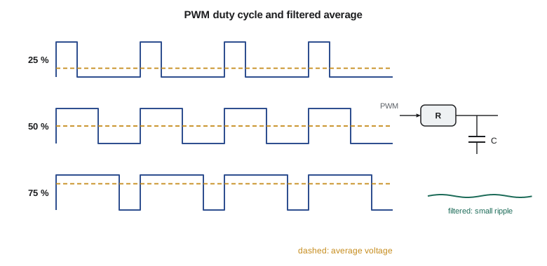
The second formula captures a trade-off. A timer clocked at 48 MHz producing a 1 kHz PWM signal counts to 48,000 each period, so the duty cycle can be set in steps of 1 in 48,000, about 15.5 bits. At 200 kHz, the same timer counts only to 240, about 7.9 bits. High PWM frequencies make filtering easier and keep the switching above the audible range for motors; low frequencies give finer resolution and lower switching losses. LED dimming needs a frequency high enough to avoid visible flicker, commonly a few hundred hertz to a few kilohertz, and fine resolution at low brightness because the eye's response is logarithmic.

Putting the analog chain together

A good analog measurement is a chain, and every link matters: the sensor and its excitation, any amplifier, the anti-aliasing filter, the source impedance seen by the ADC, the acquisition time, the reference, the converter, and the firmware's scaling, calibration and filtering. Calibration deserves its own mention. Offset and gain errors in the divider, amplifier and converter can be measured at the factory, at two known input values, and stored in flash; firmware then corrects each reading with a subtraction and a multiplication. The NS-4 production test applies 11.000 V and 14.000 V to the battery terminals and stores the resulting two-point calibration, which brings the battery measurement to within 20 mV over temperature.