
CHE-480 · Lesson 2 of 12 · 23 min
Air pollutants and dispersion
The first technical question the regulator will ask about the expansion is not how many metric tons the plant will emit, but what concentration those metric tons will cause where people live and work. The nearest house to the Cedar Rapids plant is 600 m from the fence, across a farm field, and a school sits 2.4 km downwind in the prevailing wind. Wren hands Theo a copy of the plant's last dispersion study and asks him to understand it well enough to explain it to the neighbors at the public meeting in February. This lesson covers the pollutants he will be explaining and the physics of how they spread.
Criteria pollutants and air toxics
Air pollutants are usually divided into two groups. The first are the common or criteria pollutants, which are emitted by many sources and for which governments set ambient air quality standards: fine particulate matter (PM2.5, particles smaller than 2.5 µm), coarser inhalable particles (PM10), nitrogen dioxide, sulfur dioxide, carbon monoxide, ground-level ozone and lead. In the US the ambient benchmarks are the National Ambient Air Quality Standards (NAAQS), which EPA sets under the Clean Air Act. The second group are air toxics, called hazardous air pollutants in US law: specific chemicals such as acetaldehyde, formaldehyde, acrolein, methanol, benzene and many others that can cause cancer or other serious effects at low concentrations. They are regulated chemical by chemical.
An ethanol plant emits both. Its criteria pollutants come mainly from combustion in the boilers, dryers and oxidizer, and from grain and DDGS dust. Its air toxics come from fermentation and drying: yeast and the hot drying of stillage solids produce acetaldehyde, formaldehyde, acrolein, methanol and acetic acid, mostly in small amounts. Acetaldehyde is the one that usually governs at the fermentation vent, which is why the CHE-314 scrubber design added bisulfite to the scrubbing water.
| Pollutant | Main sources at the plant | Main concern |
|---|---|---|
| PM10, PM2.5 | Dryers, grain and DDGS handling, cooling tower | Lung and heart disease, haze |
| NOx (as NO2) | Boilers, dryer burners, RTO | Respiratory effects; forms ozone and fine particles |
| SO2 | Dryers (sulfur in the feed) | Respiratory effects; acid deposition |
| CO | Dryers, boilers | Reduces oxygen carried by the blood |
| VOC | Dryers, fermentation vent, tanks, leaks | Forms ozone with NOx in sunlight |
| Acetaldehyde, formaldehyde | Fermentation vent, dryers | Irritants; probable carcinogens |
Secondary pollutants
Some of the most important pollutants are not emitted at all. Ground-level ozone forms when VOC and nitrogen oxides react in sunlight, over hours and tens of kilometers. A large share of fine particulate is secondary too: sulfur dioxide and nitrogen oxides are oxidized in the air to sulfate and nitrate, which combine with ammonia from farms to form ammonium salts. A plant's contribution to these is hard to model one source at a time, so regulators control them by limiting their precursors across a whole region. That is why VOC and nitrogen oxides are controlled even when they do not exceed any standard at the fence.
Units and conversions
Concentrations in air are given either as a volume fraction (ppm or ppb by volume) or as a mass concentration (mg/m³ or µg/m³). For an ideal gas the conversion depends on molar mass and on the temperature and pressure the volume is measured at. Ambient standards are usually stated at 25 °C and 101.325 kPa, where a mole of gas occupies 24.45 L. Stack measurements are usually corrected to a standard condition and a reference oxygen content, as Lesson 5 shows.
Worked problem
Converting an ambient concentration
A monitor at the fence records 20 ppb of nitrogen dioxide (M = 46.0 g/mol). What is this in µg/m³ at 25 °C?
Show solution
- Use the conversion at 25 °C and 1 atm, where the molar volume is 24.45 L.
- \(C = 20 \times 46.0 / 24.45 = 37.6\) µg/m³.
Answer: About 38 µg/m³.
The atmosphere as a mixing vessel
Once a pollutant leaves a stack, the wind carries it and turbulence spreads it. How much it spreads depends on the stability of the atmosphere. On a sunny afternoon the ground heats the air above it, warm parcels rise, and the air churns vigorously: the atmosphere is unstable and plumes loop down to the ground close to the stack. On a clear night with light winds the ground cools, a layer of cold air forms near the surface, and vertical motion is suppressed: the atmosphere is stable and a plume travels a long way as a thin ribbon. Overcast days and strong winds give neutral conditions in between. The Pasquill-Gifford scheme classes stability from A (very unstable) to F (very stable) using wind speed, sunshine and cloud cover, and each class has its own rate of plume spreading.
The temperature profile also decides whether a plume can mix upward at all. Normally temperature falls with height. When it rises with height, in a temperature inversion, the inversion acts as a lid. A plume released beneath a low inversion can be trapped and mixed down to the ground, which is why the worst air quality episodes often happen on still winter mornings. The depth of the layer in which pollutants mix, the mixing height, varies from a few hundred meters at night to more than a kilometer on summer afternoons.
The Gaussian plume model
The workhorse of regulatory dispersion modeling is the Gaussian plume. It treats a continuous release from a point as a plume carried downwind at the wind speed \(u\), with the concentration across the plume following a normal distribution in both the horizontal and vertical directions. The spreads are described by standard deviations \(\sigma_y\) and \(\sigma_z\), which grow with distance \(x\) at rates set by the stability class. The ground is treated as a reflecting surface, which is the same as adding an image source below the ground. The concentration at ground level on the plume centerline is then:
Here \(Q\) is the emission rate and \(H_e\) the effective stack height: the physical height plus the plume rise. Close to the stack, \(\sigma_z\) is small and the exponential term keeps the plume off the ground. Far away, the plume has spread so much that its concentration is low everywhere. In between, at a distance that grows with effective height, the ground-level concentration passes through a maximum. Doubling the effective height roughly quarters the maximum concentration, which is why tall stacks were the first tool of air pollution control.
Plume rise
A plume rises above the stack top because it is hot (buoyancy) and because it leaves the stack at speed (momentum). The equations of Briggs, used in most regulatory models, express buoyancy through a flux \(F\):
where \(v_s\) is the exit velocity, \(d\) the stack diameter and \(T_s\), \(T_a\) the stack and ambient temperatures in kelvin. For neutral and unstable conditions the final rise is about \(21.4 F^{3/4}/u\) when \(F\) is below 55 m⁴/s³ and \(38.7 F^{3/5}/u\) above it. A cold jet rises only by momentum, about \(3 d v_s / u\). A plume of carbon dioxide, which is denser than air, does not rise by buoyancy at all; if anything it tends to sink.
# Gaussian plume: plume rise and ground-level concentration downwind of two stacks
import math
g, Ta, u = 9.81, 293.0, 4.0          # ambient K, wind speed at stack top m/s
def sig(cls, x):                     # Briggs open-country coefficients, x in m
    sy = {'B': 0.16, 'C': 0.11, 'D': 0.08}[cls] * x / math.sqrt(1 + 0.0001 * x)
    sz = {'B': 0.12 * x, 'C': 0.08 * x / math.sqrt(1 + 0.0002 * x),
          'D': 0.06 * x / math.sqrt(1 + 0.0015 * x)}[cls]
    return sy, sz
def glc(Q, He, cls, x):              # ground-level centerline concentration, ug/m3 (Q in g/s)
    sy, sz = sig(cls, x)
    return 1e6 * Q / (math.pi * u * sy * sz) * math.exp(-He**2 / (2 * sz**2))
def report(name, Q, H, d, v, Ts, buoyant=True):
    if buoyant:
        F = g * v * d**2 * (Ts - Ta) / (4 * Ts)                    # buoyancy flux, m4/s3
        dh = (21.425 * F**0.75 if F < 55 else 38.71 * F**0.6) / u
    else:
        dh = 3 * d * v / u                                          # momentum rise only
    He = H + dh
    print(f"{name}: rise {dh:.0f} m, effective height {He:.0f} m")
    for cls in 'BCD':
        xm = max(range(50, 20001, 10), key=lambda x: glc(Q, He, cls, x))
        print(f"  class {cls}: max 1-h {glc(Q, He, cls, xm):6.2f} ug/m3 at {xm/1000:4.1f} km")
# RTO stack: 0.30 kg/h acetaldehyde, 45 m, 2.4 m, 18 m/s, 150 C
report('RTO stack', 0.30 / 3.6, 45, 2.4, 18, 423)
# fermentation scrubber stack, water only: 0.51 g/s acetaldehyde, 25 m, 0.49 m, 15 m/s, cool CO2
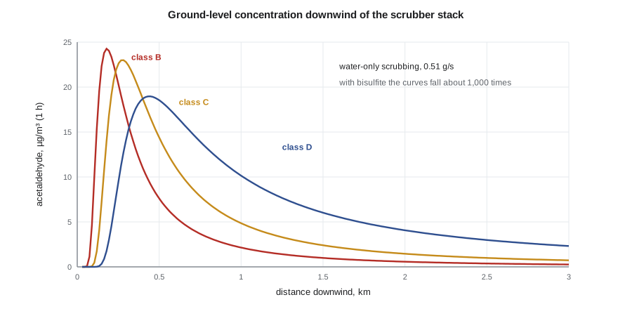
report('Scrubber stack, water only', 0.51, 25, 0.49, 15, 305, buoyant=False)RTO stack: rise 132 m, effective height 177 m class B: max 1-h 0.12 ug/m3 at 1.1 km class C: max 1-h 0.11 ug/m3 at 1.8 km class D: max 1-h 0.05 ug/m3 at 5.9 km Scrubber stack, water only: rise 6 m, effective height 31 m class B: max 1-h 24.27 ug/m3 at 0.2 km class C: max 1-h 23.01 ug/m3 at 0.3 km class D: max 1-h 18.97 ug/m3 at 0.4 km
The two stacks behave very differently. The RTO exhaust is hot and fast and leaves a 2.4 m stack, so it has a large buoyancy flux, and the plume rises more than 100 m on a moderate wind. Even with 0.30 kg/h of acetaldehyde, the highest one-hour concentration at ground level is about 0.1 µg/m³. The scrubber exhaust is cool carbon dioxide from a small stack. It rises only a few meters, and if the scrubber removed only 32 % of the acetaldehyde, as water alone would do, the highest one-hour concentration would be about 24 µg/m³ only 200 m from the stack, inside or just beyond the fence. With bisulfite the removal is better than 99.9 % and the peak falls a thousandfold. Theo sees why the CHE-314 design treated acetaldehyde as a design case, not an afterthought.
Averaging times
A one-hour Gaussian plume concentration is not directly comparable with a standard for 24 hours or a year, because the wind direction wanders. Screening methods apply factors to convert a one-hour maximum to longer averages; a factor of about 0.4 for 24 hours is common in screening work. Detailed models avoid the factor by running a whole year or more of hourly weather data and reporting the concentration at each receptor for each averaging period. The answer the regulator checks is the highest concentration, for the averaging time of the standard, at any receptor beyond the property line.
Regulatory models and what they add
In the US, compliance is judged against the NAAQS and PSD increments that Iowa DNR checks with EPA's AERMOD model, and Iowa's own review of toxic air pollutants for some sources. The Gaussian equation above is the core of the older regulatory models, but the current ones go further. EPA's AERMOD model and its equivalents describe the boundary layer with continuous variables rather than six stability classes, use five years of local hourly weather, account for terrain, and, most important for a plant like this one, model building downwash: the wake of a large building can pull a plume from a short stack down to the ground on its lee side. Building downwash is often the controlling case for short stacks near tall tanks and buildings, such as the scrubber stack beside the fermenters. Good engineering practice for stack height is about 2.5 times the height of nearby buildings; stacks shorter than that need a downwash analysis and sometimes a taller stack.
Wren uses the simple Gaussian calculation to screen. If a screening estimate is well below the standard, as it is for the RTO stack, a detailed model will almost certainly agree. If it is close, the detailed model is needed, and its answer will usually be lower but sometimes higher. Theo's water-only scrubber case is the kind of result that tells the design team to spend money on the source, not the model.
Odor
Neighbors of ethanol plants rarely complain about ozone or particulate. They complain about smell. The dryers produce a sweet, toasty odor from the browning of sugars and proteins, and the fermentation vent and the wastewater system can produce sour or sulfurous smells. Odor is measured by trained panels in odor units: the number of dilutions with clean air needed before half the panel can no longer detect it. Dispersion models can predict odor units downwind in the same way as concentrations, and some regulators set odor criteria. Wren's experience is that a good relationship with the neighbors, a complaint line that someone answers, and a log that links each complaint to the plant's operations and the weather resolve more odor problems than any model.
Ambient monitoring and the public meeting
Models are checked against measurements. Government networks run monitors for the criteria pollutants across the US, and the nearest stations give the background concentration that the plant's contribution is added to. For the expansion Wren proposes a year of on-site monitoring of PM2.5 and nitrogen dioxide at the fence nearest the houses, with a weather station, so that the dispersion study rests on local data. Theo drafts the slides for the public meeting: a map with the maximum predicted concentrations, the standards beside them, the background from the nearest station, and a plain statement of what the plant will do if a monitor shows a problem.
Common mistakes
MistakeComparing a one-hour model result directly with an annual standard.
InsteadConvert with an averaging-time factor or model a full year of weather for each averaging period.
MistakeAssuming the highest concentration is at the fence.
InsteadThe maximum is often hundreds of meters to kilometers away, farther for taller effective stacks.
MistakeTreating a cold carbon dioxide vent like a hot stack.
InsteadA cold, dense plume rises only by momentum and may sink; use momentum rise and check downwash.
MistakeUsing a tall stack instead of control.
InsteadHeight lowers ground-level concentrations but not the mass emitted; regional pollutants still need source control.
MistakeIgnoring secondary pollutants.
InsteadVOC, NOx and SO2 form ozone and fine particulate downwind; their precursors are controlled for that reason.
Summary and key terms
- Criteria pollutants have ambient standards; air toxics are regulated chemical by chemical.
- Ozone and much fine particulate are secondary, formed from precursors in the air.
- Atmospheric stability controls plume spreading; inversions trap plumes near the ground.
- The Gaussian plume model gives ground-level concentration from emission rate, wind, spreads and effective height.
- Plume rise from buoyancy and momentum can multiply the effective height of a hot stack.
- Regulatory models add real weather, terrain and building downwash; screening tells you when they are needed.
- Criteria pollutant
- A common pollutant with an ambient air quality standard, such as PM2.5, NO2, SO2, CO or ozone.
- Stability class
- A category from A to F describing how vigorously the atmosphere mixes vertically.
- Effective stack height
- Physical stack height plus plume rise.
- Buoyancy flux
- A measure of a plume's tendency to rise because it is warmer than the air.
- Building downwash
- The pulling down of a plume into the wake of a nearby building.
- Odor unit
- The number of dilutions with clean air at which half a panel can no longer detect an odor.
Practice problems
Work each problem on paper first, then reveal the answer to check.
Convert 50 ppb of SO2 (M = 64.1) to µg/m³ at 25 °C.
Show answer
\(50 \times 64.1 / 24.45 = 131\) µg/m³.
What happens to the maximum ground-level concentration if the effective height doubles?
Show answer
It falls to roughly a quarter.
Why does the scrubber plume rise so little?
Show answer
It is cool, dense carbon dioxide from a small stack, so it has only momentum rise.
Which stability class gives the highest concentration closest to a tall stack?
Show answer
Unstable classes (A or B), which loop the plume down near the source.
What is building downwash and when does it matter?
Show answer
A building wake pulling a plume down; it matters for stacks shorter than about 2.5 times nearby buildings.
Why are VOC controlled even when they meet every standard at the fence?
Show answer
They help form ozone over a region with NOx in sunlight.
Lesson quiz · 5 questions
Score 60% or more to complete this lesson.
Create a free account to save your progress, take quizzes and earn a certificate.