
CHE-260 · Lesson 3 of 12 · 24 min
Measurement statistics, calibration and quality control
The fuel ethanol specification in ASTM D4806 allows at most 0.5 percent methanol by volume. A railcar sample from Kingfisher Bioenergy measures 0.318 percent. Is that a pass? The obvious answer is yes, but Marisol pushes Theo further. How sure is the lab of 0.318? If the instrument had drifted, or the calibration were wrong, could the true value be 0.45 or 0.55? Before a lab can sign a certificate it must know not only its result but how good that result is. This lesson gives Theo the statistics to answer, and shows how calibration and routine quality control keep the answer honest day after day.
Accuracy, precision and kinds of error
Accuracy is how close a result is to the true value. Precision is how close repeated results are to each other. A method can be precise but inaccurate, giving tight results clustered around the wrong value, or imprecise but accurate on average. Good methods need both.
Errors come in three kinds. Random errors scatter results above and below the mean; they come from electronic noise, small variations in technique and the reading of scales, and they set the precision. Systematic errors push every result the same way; they come from a wrongly prepared standard, an uncalibrated pipette, an interfering substance or a biased technique, and they set the bias. Gross errors are mistakes, such as a transcription slip or a spilled sample, that make a result useless. Statistics can describe random error and help detect systematic and gross errors, but it cannot remove a bias the analyst does not know about. Only careful calibration and independent checks can do that.
Describing replicate results
For n replicate results \(x_1, x_2, \ldots, x_n\), the sample mean and sample standard deviation are:
The denominator \(n - 1\) (the degrees of freedom) corrects for the fact that the mean was estimated from the same data. The relative standard deviation, \(s/\bar{x}\) expressed as a percentage, lets methods with different units be compared. Repeatability is the precision of results obtained under the same conditions over a short time: same analyst, same instrument, same day. Reproducibility is the precision between different analysts, instruments or labs, and it is always larger. Published standard methods report both, which is how the lab knows whether its disagreement with the feed buyer's lab is normal.
When results follow a normal distribution, the mean of n results is uncertain by a confidence interval:
where t is Student's t for the chosen confidence level and \(n - 1\) degrees of freedom. For three replicates and 95 percent confidence, t = 4.30; for six replicates it is 2.57; for very many it approaches 1.96. Small numbers of replicates give wide intervals, which is why a single injection is rarely enough when a result is close to a limit.
Worked problem
Confidence interval for a water result
Five Karl Fischer measurements of water in a fuel ethanol sample give 0.348, 0.352, 0.345, 0.356 and 0.349 mass percent. Find the mean, the standard deviation and the 95 percent confidence interval.
Show solution
- Mean: the sum is 1.750, so \(\bar{x} = 0.350\) mass percent.
- Deviations: −0.002, 0.002, −0.005, 0.006, −0.001. Squares sum to \(7.0 \times 10^{-5}\).
- Standard deviation: \(s = \sqrt{7.0 \times 10^{-5}/4} = 0.0042\) mass percent.
- With 4 degrees of freedom, t = 2.78, so the half-width is \(2.78 \times 0.0042/\sqrt{5} = 0.0052\).
Answer: The water content is 0.350 ± 0.005 mass percent at 95 percent confidence.
Comparing results and spotting outliers
Statistical tests answer questions such as: does the lab's mean for a certified reference material differ from the certified value? Do two methods give the same result? A t-test compares the difference with the scatter expected from random error. If the calculated t exceeds the critical value, the difference is called statistically significant: random error alone would rarely produce it, so a systematic error is likely. An F-test compares two standard deviations to see whether one method is more precise than the other.
A result that sits far from the others may be an outlier. Before rejecting it, the analyst looks for a cause in the notebook: a bubble in the burette, a mislabeled vial. If there is none, a test such as Grubbs' test compares the suspect value's distance from the mean, in units of s, with a critical value that depends on n. Rejecting results only because they are inconvenient is a form of data manipulation, and Lesson 12 returns to why labs forbid it.
Worked problem
Testing a result against a certified reference material
The lab measures a certified reference material for water in ethanol, certified at 0.500 mass percent, six times: mean 0.509, standard deviation 0.006. Is there evidence of bias at 95 percent confidence?
Show solution
- Calculate t: \(t = |\bar{x} - \mu|\sqrt{n}/s = 0.009 \times \sqrt{6}/0.006 = 3.67\).
- The critical t for 5 degrees of freedom at 95 percent confidence is 2.57.
- Because 3.67 is larger than 2.57, the difference is statistically significant.
Answer: The method reads about 0.009 mass percent high, a real bias. The lab checks the titrant factor and the drift correction before using the method on customer samples.
Significant figures and rounding
A result should be reported with as many digits as the uncertainty justifies, no more. If the uncertainty is ±0.005, reporting 0.31842 implies a precision the method does not have; 0.318 is right. A useful rule is to round the uncertainty to one or two significant figures and then round the result to the same decimal place. Calculations should carry extra digits and round only at the end, because rounding at each step adds error. Specifications usually state how results are compared with limits, for example by rounding to the number of digits in the limit before comparing, and the lab follows that rule exactly so that two labs reach the same pass or fail decision from the same data.
Calibration
Most instruments do not measure concentration directly. A gas chromatograph gives peak areas, a spectrophotometer gives absorbance, a plasma instrument gives emission counts. Calibration is the process of relating the instrument response to known concentrations. The analyst prepares a set of standards spanning the expected range, measures them, and fits a line by the method of least squares, which chooses the slope b and intercept a that minimize the sum of squared vertical deviations:
The standard error of the regression, \(s_y = \sqrt{\sum (y_i - a - bx_i)^2/(n-2)}\), measures how far points scatter from the line. The correlation coefficient r is often quoted, but a value of 0.999 does not by itself prove a good calibration: a slightly curved response can still give r above 0.999. The better check is to look at the residuals. If they wander randomly around zero, a straight line fits; if they curve or grow with concentration, the line is wrong and the analyst should narrow the range, use a weighted fit or fit a curve.
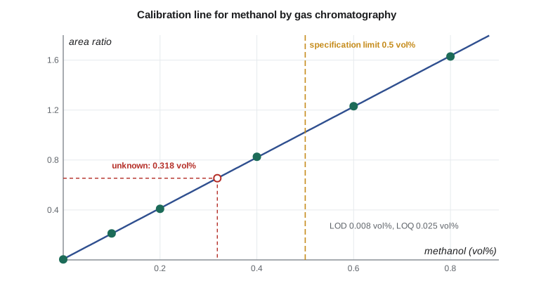
Unknowns must fall within the calibrated range. Extrapolating beyond the highest standard assumes the line continues straight, which detectors often do not. A sample that reads above the top standard is diluted and run again. The calibration also has an uncertainty, so a concentration read from it carries an interval that depends on the scatter of the calibration, the number of standards, the number of replicate readings of the unknown and how far the unknown lies from the center of the calibration.
Detection and quantitation limits
Every method has a lower limit below which it cannot reliably tell a small amount of analyte from none. The limit of detection (LOD) is the smallest concentration that gives a signal distinguishable from the blank with reasonable confidence. The limit of quantitation (LOQ) is the smallest concentration that can be measured with acceptable precision. Common estimates use the standard deviation of blank signals, or the standard error of a low-level calibration, divided by the slope:
Results between the LOD and LOQ are reported as detected but not quantified, and results below the LOD as less than the LOD, never as zero. For the methanol method, both limits are far below the specification limit, so the method is fit for purpose. For copper at a fraction of a milligram per kilogram, the LOD matters much more, which is one reason the lab uses a plasma instrument for metals (Lesson 8).
Working through a calibration
The program below fits the methanol calibration Theo ran on the gas chromatograph, estimates the detection limits, and reads three replicate injections of the railcar sample with a 95 percent confidence interval.
# Calibration line, detection limits and an unknown: methanol in fuel ethanol by GC
import math

conc = [0.00, 0.10, 0.20, 0.40, 0.60, 0.80]           # methanol, vol%
resp = [0.004, 0.212, 0.409, 0.826, 1.231, 1.629]      # peak-area ratio to internal standard
n = len(conc)
xm = sum(conc) / n; ym = sum(resp) / n
Sxx = sum((x - xm) ** 2 for x in conc)
Sxy = sum((x - xm) * (y - ym) for x, y in zip(conc, resp))
b = Sxy / Sxx; a = ym - b * xm
res = [y - (a + b * x) for x, y in zip(conc, resp)]
sy = math.sqrt(sum(r * r for r in res) / (n - 2))
r = Sxy / math.sqrt(Sxx * sum((y - ym) ** 2 for y in resp))
print(f"slope = {b:.4f} per vol%, intercept = {a:.4f}, r = {r:.5f}")
print(f"standard error of the regression s_y = {sy:.4f}")

# Detection and quantitation limits from the calibration (3.3 s/b and 10 s/b)
LOD = 3.3 * sy / b; LOQ = 10 * sy / b
print(f"LOD = {LOD:.3f} vol%, LOQ = {LOQ:.3f} vol%")

# Unknown: three replicate injections of a production sample
y0 = [0.652, 0.661, 0.648]
m = len(y0); ybar = sum(y0) / m
x0 = (ybar - a) / b
sx0 = sy / b * math.sqrt(1 / m + 1 / n + (ybar - ym) ** 2 / (b * b * Sxx))
t = 2.776   # Student t, 95 %, 4 degrees of freedom
print(f"methanol = {x0:.3f} +/- {t * sx0:.3f} vol% (95 % confidence)")
print("meets the 0.5 vol% limit:", x0 + t * sx0 < 0.5)slope = 2.0344 per vol%, intercept = 0.0065, r = 0.99997 standard error of the regression s_y = 0.0051 LOD = 0.008 vol%, LOQ = 0.025 vol% methanol = 0.318 +/- 0.005 vol% (95 % confidence) meets the 0.5 vol% limit: True
The result is 0.318 ± 0.005 percent methanol. Even the upper end of the interval is far below 0.5 percent, so the lab can certify the car with confidence. Had the result been 0.497 ± 0.005, the decision would be much harder, and the lab's written decision rule would say how to handle it.
Quality control in routine work
Calibration shows a method works on the day it is calibrated. Quality control shows it keeps working. Routine QC samples are run with every batch of unknowns:
| QC sample | What it detects |
|---|---|
| Reagent or method blank | Contamination and baseline drift |
| Check standard (calibration verification) | Drift in the calibration since it was set up |
| Duplicate sample | Loss of precision |
| Spiked sample | Matrix effects and losses during preparation |
| Certified reference material | Bias against an independently certified value |
Results for a check standard are plotted on a control chart, a running record with the target value as the center line and warning and action limits, usually at ±2s and ±3s, where s comes from the method's long-term performance. About 95 percent of results should fall within the warning limits by chance. Simple rules, adapted from clinical labs, flag problems: one result beyond the action limits means stop and investigate; two consecutive results beyond the same warning limit, or four in a row more than 1s on the same side of the target, suggest a systematic shift such as a degrading standard or a drifting detector.
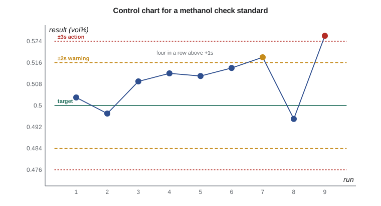
Theo's control chart showed exactly that pattern. Four check standards in a row sat above +1s before one crossed the action limit. The cause was a check standard that had been left uncapped and was slowly losing ethanol by evaporation, which concentrated its methanol. The control chart caught it before any customer results were affected, which is its whole purpose.
Common mistakes
MistakeTreating r = 0.999 as proof of a straight-line calibration.
InsteadPlot the residuals; curvature can hide behind a high r.
MistakeReporting a result below the LOD as zero.
InsteadReport it as less than the LOD.
MistakeReading an unknown that lies above the highest standard.
InsteadDilute it into the calibrated range and run it again.
MistakeDeleting a result because it looks odd.
InsteadLook for a documented cause; otherwise use a recognized test and record what was done.
Summary and key terms
- Accuracy is closeness to the true value; precision is closeness of replicates. Random errors set precision and systematic errors set bias.
- The mean, standard deviation and Student's t give a confidence interval for the true value.
- Least-squares calibration relates instrument response to concentration; check the residuals, not just r.
- LOD and LOQ are about 3.3s/b and 10s/b; report results below the LOD as less than the LOD.
- Blanks, check standards, duplicates, spikes and reference materials run with every batch.
- Control charts with ±2s and ±3s limits and simple run rules reveal drift before it affects results.
- Accuracy
- Closeness of a result to the true value.
- Precision
- Closeness of repeated results to each other.
- Systematic error
- An error that biases all results in the same direction.
- Repeatability
- Precision under the same conditions over a short time.
- Reproducibility
- Precision between different analysts, instruments or laboratories.
- Calibration
- Establishing the relation between instrument response and known amounts of analyte.
- Limit of detection
- The smallest concentration that can be distinguished from a blank with reasonable confidence.
- Control chart
- A plot of quality control results against time with limits that signal when a method is out of control.
Practice problems
Work each problem on paper first, then reveal the answer to check.
Three results are 12.1, 12.4 and 12.2 g/L. Find the mean and standard deviation.
Show answer
Mean 12.23 g/L; s = 0.15 g/L.
For those three results, what is the 95 percent confidence interval (t = 4.30)?
Show answer
\(12.23 \pm 4.30 \times 0.15/\sqrt{3} = 12.23 \pm 0.38\) g/L.
A calibration has slope 2.03 per vol% and s = 0.0051. Estimate the LOQ.
Show answer
\(10 \times 0.0051/2.03 = 0.025\) vol%.
Why should a calibration not be extrapolated above the top standard?
Show answer
The response may curve at high concentration, so the line may no longer hold.
What does a spiked sample reveal that a check standard does not?
Show answer
Effects of the sample matrix, such as suppression or losses during preparation.
Two consecutive check standards fall between +2s and +3s. What should the analyst do?
Show answer
Treat it as a likely systematic shift: stop, investigate the standard and instrument, and rerun before reporting.
Lesson quiz · 5 questions
Score 60% or more to complete this lesson.
Create a free account to save your progress, take quizzes and earn a certificate.