
CHE-250 · Lesson 9 of 12 · 25 min
Rate laws and integrated rate equations
Thermodynamics tells Theo which way a reaction can go and how far it can get. It says nothing about how long that takes. Ethanol and oxygen have a huge negative Gibbs energy of reaction, yet ethanol sits safely in storage tanks for months. The starch in corn would hydrolyze to glucose eventually, but without enzymes the plant would wait years for each batch. Chemical kinetics, the study of reaction rates, is the other half of reactor design, and at Kingfisher Bioenergy it governs how long the fermenters run, how much enzyme is dosed, how fast contaminants build up and how long a catalyst lasts. The next three lessons develop it: rate laws in this lesson, the effect of temperature in Lesson 10 and mechanisms and catalysis in Lesson 11.
Theo begins in the quality lab. A technician has measured how fast ethyl acetate is hydrolyzed by sodium hydroxide, a classic kinetics experiment that the lab also uses to check the strength of its caustic solutions. Ingrid asks Theo to find the order of the reaction and its rate constant from the data, and then to apply the same thinking to the plant's liquefaction enzymes, which slowly lose activity in the hot mash.
Defining the rate of reaction
For a reaction \(a\text{A} + b\text{B} \to c\text{C} + d\text{D}\) in a closed vessel of constant volume, the rate is defined so that it is the same whichever species is followed:
Dividing by the stoichiometric coefficients removes the ambiguity: if two moles of A are used for every mole of C formed, A disappears twice as fast as C appears, but the reaction rate is one number. Rates are usually expressed in mol/(L s) for solutions. In a flowing reactor the definition is written per unit volume of reactor, which CHE-345 Chemical Reaction Engineering develops for real reactor types; here we stay with well-mixed batch systems, which are what the lab and the fermenters are.
Rate laws, orders and rate constants
Experiments show that the rate of most reactions depends on concentrations through a rate law of the form:
The exponents \(\alpha\) and \(\beta\) are the orders with respect to A and B, and their sum is the overall order. The rate constant \(k\) depends on temperature but not on concentration. Orders must be found by experiment. They are often small integers, but they need not match the stoichiometric coefficients, and they can be fractions or even negative. Only for an elementary reaction, a single molecular step, do the orders equal the coefficients, as Lesson 11 explains. The units of \(k\) depend on the overall order: s⁻¹ for first order, L/(mol s) for second order, and mol/(L s) for zero order.
| Overall order | Rate law | Units of k | Example |
|---|---|---|---|
| Zero | \(r = k\) | mol/(L s) | Enzyme reaction at saturating substrate |
| First | \(r = k[\text{A}]\) | s⁻¹ | Radioactive decay; enzyme deactivation |
| Second | \(r = k[\text{A}]^2\) or \(k[\text{A}][\text{B}]\) | L/(mol s) | Ester hydrolysis by hydroxide |
| Fractional | \(r = k[\text{A}]^{3/2}\) | (L/mol)^½/s | Some chain reactions |
The method of initial rates
One way to find the orders is to measure the rate at the very start of a reaction, before concentrations change much, in a series of runs with different starting concentrations. Doubling the concentration of A while holding B fixed doubles the rate if the reaction is first order in A, quadruples it if second order, and leaves it unchanged if zero order. In general, the order is \(\alpha = \ln(r_2/r_1)/\ln([\text{A}]_2/[\text{A}]_1)\).
Worked problem
Orders from initial rates
Three runs give these initial rates: [A] = 0.10 and [B] = 0.10 mol/L, rate \(2.0 \times 10^{-4}\); [A] = 0.20, [B] = 0.10, rate \(4.0 \times 10^{-4}\); [A] = 0.10, [B] = 0.20, rate \(8.0 \times 10^{-4}\) mol/(L s). Find the orders and the rate constant.
Show solution
- Runs 1 and 2: doubling [A] doubles the rate, so \(\alpha = \ln 2/\ln 2 = 1\).
- Runs 1 and 3: doubling [B] quadruples the rate, so \(\beta = \ln 4/\ln 2 = 2\).
- Rate law: \(r = k[\text{A}][\text{B}]^2\). From run 1: \(k = 2.0 \times 10^{-4}/(0.10 \times 0.10^2) = 0.20\) L²/(mol² s).
Answer: First order in A, second order in B, third order overall, with k = 0.20 L²/(mol² s).
Integrated rate laws
The method of initial rates needs several runs. Following a single run over time is often easier, and it requires integrating the rate law to give concentration as a function of time. For a reaction \(\text{A} \to \text{products}\) the three common cases are:
| Order | Integrated form | Linear plot | Half-life |
|---|---|---|---|
| Zero | \([\text{A}] = [\text{A}]_0 - kt\) | \([\text{A}]\) against \(t\), slope \(-k\) | \([\text{A}]_0/(2k)\) |
| First | \(\ln[\text{A}] = \ln[\text{A}]_0 - kt\) | \(\ln[\text{A}]\) against \(t\), slope \(-k\) | \(\ln 2/k\) |
| Second | \(1/[\text{A}] = 1/[\text{A}]_0 + kt\) | \(1/[\text{A}]\) against \(t\), slope \(k\) | \(1/(k[\text{A}]_0)\) |
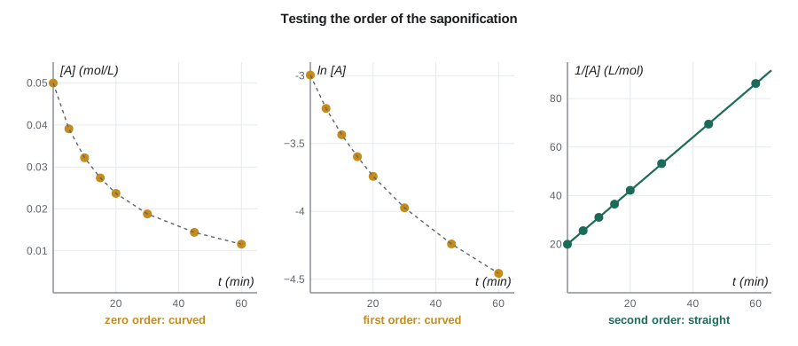
The integrated forms give a practical test for order: plot the data three ways and see which gives a straight line. The slope of that line gives the rate constant. For a second-order reaction between two different species, \(\text{A} + \text{B} \to\) products with \(r = k[\text{A}][\text{B}]\), starting with equal concentrations makes \([\text{A}] = [\text{B}]\) at all times, so the simple second-order form applies. With unequal concentrations the integrated law is more complicated, or the experimenter uses a large excess of one reactant so that its concentration hardly changes; the reaction then behaves as pseudo-first order in the other.
Half-lives
The half-life, the time for a reactant's concentration to fall to half its starting value, behaves differently for each order and offers another quick test. For a first-order reaction, \(t_{1/2} = \ln 2/k\) does not depend on concentration: every half-life is the same length, whether the concentration is falling from 1 to 0.5 mol/L or from 0.01 to 0.005. For a second-order reaction, \(t_{1/2} = 1/(k[\text{A}]_0)\), so each successive half-life is twice as long as the one before, because the molecules have fewer partners to react with. For a zero-order reaction each half-life is half as long as the one before.
First-order kinetics is especially common because any process in which each molecule has a fixed probability of reacting per unit time is first order. Radioactive decay, the loss of activity of an enzyme held at high temperature, the death of microorganisms during sterilization and the decay of many drugs in the body all follow it. Constant half-lives make first-order processes easy to reason about: after ten half-lives, less than 0.1 percent remains.
Worked problem
Enzyme activity in the liquefaction tank
The plant's alpha-amylase loses activity in the hot liquefaction tank by first-order deactivation with an illustrative rate constant of 0.0231 min⁻¹. Find its half-life and the fraction of activity left after the 90-minute residence time.
Show solution
- \(t_{1/2} = \ln 2/k = 0.693/0.0231 = 30\) min.
- After 90 min, three half-lives: fraction remaining \(= e^{-0.0231 \times 90} = e^{-2.08} = 0.125\), or 12.5 percent.
Answer: A 30-minute half-life, with an eighth of the activity left after 90 minutes. That is why the enzyme is dosed in two stages, part before the jet cooker and part after, and why choosing a more heat-stable enzyme can cut enzyme costs substantially. Lesson 10 shows why a few degrees of temperature change this rate constant so much.
Finding the order from a single run
The lab's saponification data illustrate the graphical method. Sodium hydroxide and ethyl acetate were mixed at equal initial concentrations of 0.0500 mol/L, and the hydroxide concentration was followed by conductivity. The program below fits the data as zero-, first- and second-order reactions by least squares and reports the coefficient of determination, \(R^2\), for each. It then works out the half-lives, the enzyme deactivation example and the initial-rates example.
# Finding the order of a reaction from concentration-time data by linear regression
import math

def fit(x, y):
    n = len(x); mx = sum(x) / n; my = sum(y) / n
    sxx = sum((a - mx) ** 2 for a in x); sxy = sum((a - mx) * (b - my) for a, b in zip(x, y))
    m = sxy / sxx; c = my - m * mx
    ss_res = sum((b - (m * a + c)) ** 2 for a, b in zip(x, y)); ss_tot = sum((b - my) ** 2 for b in y)
    return m, c, 1 - ss_res / ss_tot

# saponification of ethyl acetate with NaOH, equal initial concentrations (illustrative lab data)
t = [0, 5, 10, 15, 20, 30, 45, 60]                       # min
C = [0.0500, 0.0391, 0.0322, 0.0274, 0.0237, 0.0188, 0.0144, 0.0116]   # mol/L of NaOH
tests = {'zero order  (C vs t)':     [c for c in C],
         'first order (ln C vs t)':  [math.log(c) for c in C],
         'second order (1/C vs t)':  [1 / c for c in C]}
for name, y in tests.items():
    m, c0, r2 = fit(t, y)
    print(f"{name:26s} slope = {m:10.5f}  R^2 = {r2:.4f}")
k2 = fit(t, [1 / c for c in C])[0]
print(f"second-order rate constant k = {k2:.3f} L/(mol min)")
print(f"first half-life = {1 / (k2 * C[0]):.1f} min; from 0.025 M the next half-life = {1 / (k2 * 0.025):.1f} min")

# first-order example: thermal loss of enzyme activity in a hot liquefaction tank
kd = 0.0231   # 1/min, illustrative
print(f"\nenzyme half-life = {math.log(2) / kd:.0f} min; activity left after 90 min = {100 * math.exp(-kd * 90):.1f}%")

# method of initial rates: rate = k [A]^a [B]^b
runs = [(0.10, 0.10, 2.0e-4), (0.20, 0.10, 4.0e-4), (0.10, 0.20, 8.0e-4)]   # [A], [B], rate (mol/(L s))
a = math.log(runs[1][2] / runs[0][2]) / math.log(runs[1][0] / runs[0][0])
b = math.log(runs[2][2] / runs[0][2]) / math.log(runs[2][1] / runs[0][1])
k = runs[0][2] / (runs[0][0] ** a * runs[0][1] ** b)
print(f"initial rates: order in A = {a:.1f}, order in B = {b:.1f}, k = {k:.3g} (L/mol)^{a + b - 1:.0f}/s")zero order (C vs t) slope = -0.00057 R^2 = 0.8315 first order (ln C vs t) slope = -0.02348 R^2 = 0.9568 second order (1/C vs t) slope = 1.10169 R^2 = 1.0000 second-order rate constant k = 1.102 L/(mol min) first half-life = 18.2 min; from 0.025 M the next half-life = 36.3 min enzyme half-life = 30 min; activity left after 90 min = 12.5% initial rates: order in A = 1.0, order in B = 2.0, k = 0.2 (L/mol)^2/s
Only the second-order plot is straight, with \(R^2\) essentially equal to 1 and a rate constant of about 1.1 L/(mol min) for these illustrative data. The first half-life is about 18 minutes and the next is about 36 minutes, doubling as a second-order reaction should. A caution on fitting: an \(R^2\) of 0.96 for the first-order plot might look acceptable on its own. Always compare the alternatives and look at the residuals, the scatter of points about the line; a systematic curve in the residuals is the signature of the wrong model.
Following a reaction in the lab
Kinetic data are only as good as the concentration measurements behind them. The method must be fast compared with the reaction and must not disturb it. Physical methods that follow a property proportional to concentration are best, because they can be read continuously: conductivity for reactions that consume or produce ions, as in the saponification here, where highly mobile hydroxide ions are replaced by slower acetate ions; absorbance of light at a wavelength where one species absorbs; pressure for gas reactions that change the number of moles. Chemical methods, such as titration or gas chromatography of withdrawn samples, need the reaction in each sample to be stopped, or quenched, instantly by cooling, dilution or neutralization, so that the measured concentration is the one at the sampling time.
Temperature control matters as much as the analysis. Lesson 10 shows that a rate constant can change by 10 percent or more per kelvin, so kinetics experiments are run in thermostatted baths held within about 0.1 K. A data set collected while the temperature drifted will curve on every plot and can fool the analyst into choosing the wrong order.
Reversible reactions and the approach to equilibrium
Many reactions do not go to completion, and their rate laws must include the reverse reaction. For a simple reversible first-order reaction \(\text{A} \xrightleftharpoons{} \text{B}\), with forward rate constant \(k_f\) and reverse rate constant \(k_r\), the net rate is \(k_f[\text{A}] - k_r[\text{B}]\). Integrating shows that the concentration of A approaches its equilibrium value exponentially, with an observed rate constant equal to the sum \(k_f + k_r\). At equilibrium the net rate is zero, so \(k_f[\text{A}]_{eq} = k_r[\text{B}]_{eq}\), which gives:
This is the bridge between kinetics and the thermodynamics of Lesson 4: the equilibrium constant is the ratio of the forward and reverse rate constants. A catalyst speeds up both directions by the same factor, so it leaves K unchanged, exactly as Lesson 4 stated. The esterification of acetic acid with ethanol behaves this way, approaching its equilibrium of about two-thirds conversion along a curve whose rate depends on both the forward and the reverse reaction.
Kinetics in a fermenter
Fermentation itself does not follow a simple rate law, because the catalyst, the yeast, grows as it works. Early in a batch, yeast cells multiply roughly exponentially, a first-order process in cell concentration. As glucose falls, ethanol accumulates and inhibits the yeast, and the rate slows. Biochemical engineers model this with growth equations such as the Monod equation, which has the same form as the Michaelis-Menten law for enzymes in Lesson 11. The tools of this lesson still apply to the pieces: the decay of contaminating bacteria under heat, the deactivation of enzymes, and the hydrolysis of esters in the beer column all follow simple rate laws.
Common mistakes
MistakeAssuming reaction orders equal stoichiometric coefficients.
InsteadOrders must be measured; they match the coefficients only for elementary steps.
MistakeForgetting the units of the rate constant change with order.
InsteadCheck them: s⁻¹ for first order, L/(mol s) for second order.
MistakeUsing the first-order half-life formula for every reaction.
InsteadOnly first-order half-lives are independent of concentration.
MistakeChoosing a model from one plot's R² alone.
InsteadCompare all candidate plots and inspect the residuals for curvature.
Summary and key terms
- The rate of reaction is defined per stoichiometric coefficient, so it is the same for every species.
- Rate laws r = k[A]^α[B]^β have orders found by experiment and a temperature-dependent rate constant.
- The method of initial rates finds each order from how the starting rate changes with one concentration.
- Integrated laws: [A] linear in t (zero order), ln[A] linear (first), 1/[A] linear (second).
- First-order half-lives are constant, ln 2/k; second-order half-lives double as the reaction proceeds.
- Pseudo-first-order conditions use a large excess of one reactant to simplify a second-order reaction.
- Rate of reaction
- The rate of change of concentration divided by the stoichiometric coefficient.
- Rate law
- An equation giving the reaction rate as a function of concentrations.
- Reaction order
- The exponent of a concentration in the rate law.
- Rate constant
- The proportionality constant k in a rate law, which depends on temperature.
- Integrated rate law
- An equation giving concentration as a function of time, obtained by integrating the rate law.
- Half-life
- The time for a reactant's concentration to fall to half its starting value.
- Pseudo-first-order reaction
- A higher-order reaction run with a large excess of one reactant so that it appears first order.
- Method of initial rates
- Finding orders by comparing initial rates in runs with different starting concentrations.
Practice problems
Work each problem on paper first, then reveal the answer to check.
A first-order reaction has k = 0.0050 s⁻¹. What is its half-life?
Show answer
\(0.693/0.0050 = 139\) s.
For the same reaction, what fraction remains after 10 minutes?
Show answer
\(e^{-0.0050 \times 600} = e^{-3} = 0.050\), or 5 percent.
A second-order reaction with k = 0.50 L/(mol s) starts at 0.10 mol/L. What is the concentration after 60 s?
Show answer
\(1/[\text{A}] = 10 + 0.50 \times 60 = 40\), so [A] = 0.025 mol/L.
What are the units of k for a third-order reaction?
Show answer
L²/(mol² s).
Doubling a reactant's concentration leaves the initial rate unchanged. What is the order in that reactant?
Show answer
Zero.
Why might ethyl acetate hydrolysis be run with a large excess of hydroxide?
Show answer
To make the reaction pseudo-first order in ethyl acetate, which simplifies the analysis.
Lesson quiz · 5 questions
Score 60% or more to complete this lesson.
Create a free account to save your progress, take quizzes and earn a certificate.