
CHE-230 · Lesson 8 of 12 · 21 min
Flow measurement
A water utility runs on its flow measurements. They bill customers, pace chemical feed, check pump performance and reveal leaks. The incoming main at Northside carries a venturi meter installed when the station was built, and a newer magnetic meter was added on the discharge header in a recent upgrade. When the two disagreed by four percent last spring, Hana Lindqvist asked Jun Park to find out which was right. Doing that requires understanding how each meter works, what assumptions its calibration rests on and how installation affects it. This lesson covers the main families of flow meters, with emphasis on the differential-pressure meters that come straight from the Bernoulli and continuity equations.
Obstruction meters: the common principle
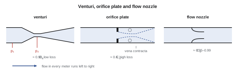
A venturi, a flow nozzle and an orifice plate all work the same way. They force the flow through a reduced area, where it speeds up, and the pressure drops. Measuring the pressure difference between the upstream pipe and the throat gives the velocity, and hence the flow rate. Combining continuity, \(V_1 A_1 = V_2 A_2\), with Bernoulli between section 1 in the pipe and section 2 at the throat gives the ideal flow rate. The diameter ratio \(\beta = d/D\) appears through the area ratio.
Real meters deliver less than the ideal value, for two reasons. Friction between the taps causes a small loss, and in an orifice the jet keeps contracting after it passes through the plate, so the true minimum area, the vena contracta, is smaller than the hole. Both effects are covered by an experimentally determined discharge coefficient \(C_d\), defined as actual flow divided by ideal flow. Meter standards, such as ISO 5167 and the corresponding ASME standards, give \(C_d\) as a function of \(\beta\) and the Reynolds number for meters built to specified dimensions.
The square root in this equation has a practical consequence. Flow is proportional to the square root of the differential pressure, so a meter whose transmitter spans 0 to 50 kPa reads half of full flow at only a quarter of full differential, 12.5 kPa. At low flows the differential becomes tiny, and the measurement loses accuracy. A single differential-pressure meter usually covers a turndown of only about 4 to 1 with good accuracy, which is one reason utilities moved to other technologies for meters that must cover a wide range of flows.
The venturi meter
A venturi has a conical inlet that contracts at about 21° to a short cylindrical throat, followed by a long diffuser that expands at 7° to 15° back to the pipe diameter. The smooth contraction gives a discharge coefficient near 0.98, almost independent of Reynolds number in turbulent flow, and the gentle diffuser recovers most of the pressure drop, so the permanent loss is only about 10 to 15 percent of the measured differential. That low loss makes the venturi the traditional choice for large water mains, where every kilopascal lost must be supplied by pumping energy for decades. Its drawbacks are length and cost.
Worked problem
Flow through the venturi on the incoming main
The venturi on the 600 mm (24 in) incoming main has a 360 mm (14.2 in) throat and \(C_d = 0.985\). The differential pressure transmitter reads 20.0 kPa (2.90 psi). Find the flow rate in m³/s and gpm.
Show solution
- \(\beta = 360/600 = 0.60\); \(\beta^4 = 0.1296\); throat area \(A_2 = \pi(0.360)^2/4 = 0.1018\ \text{m}^2\).
- \(Q = 0.985(0.1018)\sqrt{2(20\,000)/(998 \times 0.8704)} = 0.1003\sqrt{46.05}\).
- \[Q = 0.680\ \text{m}^3/\text{s} = 10\,780\ \text{gpm}\]
Answer: The main carries 680 L/s, which is an average velocity of 2.4 m/s in the 600 mm pipe. Throat velocity is 6.7 m/s; the Reynolds number in the pipe is about 1.4 million, well into the range where the venturi coefficient is constant.
The orifice plate
An orifice plate is a thin plate with a sharp-edged hole, clamped between two flanges. It is cheap, compact and easy to replace or resize, which makes it the most common flow meter in process industries. The price is a large permanent pressure loss: the jet leaving the hole separates, and its kinetic energy is mostly dissipated in eddies downstream. For \(\beta = 0.6\), the permanent loss is about 60 percent of the measured differential. Its discharge coefficient is about 0.6 and depends somewhat on Reynolds number and on where the pressure taps are placed: flange taps, corner taps or taps one diameter upstream and half a diameter downstream.
The program below compares a venturi and an orifice of the same diameter ratio in the 600 mm main. Because the orifice's discharge coefficient is lower, the same differential corresponds to much less flow, about 62 percent of the venturi's. Turn that around: to pass the same flow, the orifice needs about 2.6 times the differential, and most of that becomes permanent loss. On a large main pumped around the clock, that loss would cost thousands of dollars a year in electricity, which is why orifices are reserved for small lines and temporary tests.
# Flow measurement: venturi and orifice meters with a Reynolds-number-dependent discharge coefficient
import math
rho, mu = 998.0, 1.0e-3

def meter_flow(dp, D, d, Cd_fn, tol=1e-10):
    beta = d / D
    A2 = math.pi * d**2 / 4
    Cd = 0.6
    for _ in range(50):
        Q = Cd * A2 * math.sqrt(2 * dp / (rho * (1 - beta**4)))
        Re = rho * (Q / (math.pi * D**2 / 4)) * D / mu
        new = Cd_fn(beta, Re)
        if abs(new - Cd) < tol: break
        Cd = new
    return Q, Cd, Re

venturi = lambda beta, Re: 0.985                      # nearly constant in turbulent flow
def orifice(beta, Re):                                 # Reader-Harris/Gallagher form, corner taps, simplified
    return 0.5961 + 0.0261 * beta**2 - 0.216 * beta**8 + 0.000521 * (1e6 * beta / Re) ** 0.7 \
        + (0.0188 + 0.0063 * (19000 * beta / Re) ** 0.8) * (1e6 / Re) ** 0.3 * beta**3.5

D, d = 0.600, 0.360
for dp_kPa in (5.0, 20.0, 45.0):
    Qv, Cv, Re = meter_flow(dp_kPa * 1e3, D, d, venturi)
    Qo, Co, _ = meter_flow(dp_kPa * 1e3, D, d, orifice)
    print(f"dp = {dp_kPa:4.1f} kPa: venturi Q = {Qv*1000:6.1f} L/s (Cd {Cv:.3f}),"
          f" orifice Q = {Qo*1000:6.1f} L/s (Cd {Co:.3f}), Re = {Re:,.0f}")

# Permanent pressure loss: roughly 10 % of dp for a venturi, (1 - beta^1.9) of dp for an orifice
beta = d / D
print(f"Permanent loss, orifice: {(1 - beta**1.9)*100:.0f} % of dp; venturi: about 10 % of dp")dp = 5.0 kPa: venturi Q = 340.2 L/s (Cd 0.985), orifice Q = 209.5 L/s (Cd 0.607), Re = 720,437 dp = 20.0 kPa: venturi Q = 680.4 L/s (Cd 0.985), orifice Q = 418.3 L/s (Cd 0.606), Re = 1,440,873 dp = 45.0 kPa: venturi Q = 1020.5 L/s (Cd 0.985), orifice Q = 626.9 L/s (Cd 0.605), Re = 2,161,310 Permanent loss, orifice: 62 % of dp; venturi: about 10 % of dp
The orifice calculation must iterate, because the discharge coefficient depends on the Reynolds number, which depends on the flow, which depends on the coefficient. The loop converges in a few passes. This kind of fixed-point iteration appears throughout pipe-flow work, most importantly in the Colebrook equation for friction in Lesson 11.
Flow nozzles and installation effects
A flow nozzle sits between the venturi and the orifice: a short, rounded entrance contracting to a cylindrical throat, without the long diffuser. Its discharge coefficient is high, about 0.95 to 0.99, and it resists erosion, so it is common in high-velocity steam and boiler feedwater lines. Its permanent loss is between those of the venturi and the orifice.
All obstruction meters assume a fully developed, swirl-free velocity profile entering them, and their coefficients are valid only if that is true. Elbows, valves and pumps upstream distort the profile and add swirl, shifting the reading by several percent. Standards specify minimum straight lengths, often 10 to 40 pipe diameters upstream and 5 downstream, depending on the fitting and the diameter ratio. Where space is short, a flow conditioner, a perforated plate or a bundle of tubes, is installed to straighten the flow. Jun found that the magnetic meter at Northside was only three diameters downstream of a pair of elbows in different planes, a classic source of swirl, and that explained most of the four percent discrepancy.
Velocity-based and other meters
Several meters measure velocity directly. A pitot traverse, measuring velocity at a grid of points across a pipe and averaging, is the classic field method for checking large meters. An insertion meter uses one probe at a representative point. Magnetic flow meters exploit Faraday's law: water is a weak conductor, so as it moves through a magnetic field across the pipe, it generates a voltage between two electrodes proportional to the average velocity. Magnetic meters have no obstruction and no pressure loss, measure flow in either direction and cover a turndown of 100 to 1 or more, which has made them the standard choice for new water and wastewater installations.
Ultrasonic transit-time meters send sound pulses diagonally across the pipe, first downstream and then upstream. The pulse traveling with the flow arrives sooner, and the time difference gives the average velocity along the path. Clamp-on versions mount on the outside of the pipe, which makes them ideal for temporary checks like Jun's. Turbine meters, with a bladed rotor spinning at a speed proportional to velocity, and positive-displacement meters, which trap and count discrete volumes, dominate customer metering: the meter on each house is usually a positive-displacement or multi-jet design. Each type has its own accuracy curve, sensitivity to installation, maintenance needs and cost.
| Meter | Typical accuracy | Permanent loss | Typical use |
|---|---|---|---|
| Venturi | ±0.5–1 % | Low (10–15 % of Δp) | Large water mains |
| Orifice plate | ±1–2 % | High (40–70 % of Δp) | Process lines, temporary tests |
| Flow nozzle | ±1 % | Medium | Steam, feedwater |
| Magnetic | ±0.2–0.5 % | None | Water and wastewater, slurries |
| Ultrasonic transit-time | ±0.5–2 % | None | Large pipes, clamp-on checks |
| Positive displacement | ±1.5 % at low flow | Moderate | Customer meters |
Open-channel measurement
Not all flow is in full pipes. Raw water arriving in an intake channel, wastewater in a sewer and backwash water in a launder all flow with a free surface. Weirs and flumes measure these flows. A sharp-crested weir is a plate across the channel; water spills over its crest, and the depth of water upstream, the head, sets the flow. For a rectangular weir, Bernoulli applied to elemental strips of the nappe gives a flow proportional to the head to the power 1.5; for a V-notch weir it goes as the head to the power 2.5, which gives good resolution at low flows. A Parshall flume is a shaped channel contraction that forces the flow through critical depth, so a single upstream depth reading gives the flow without the large head loss of a weir. Open-channel hydraulics is covered fully in a later course.
Common mistakes
MistakeUsing the ideal flow equation without a discharge coefficient.
InsteadMultiply by C_d: about 0.98 for a venturi and 0.6 for an orifice.
MistakeAssuming flow is proportional to differential pressure.
InsteadQ ∝ √Δp; half the flow gives a quarter of the differential.
MistakeTreating the measured differential across an orifice as its pressure loss.
InsteadThe permanent loss is less than Δp: about 60 % for β = 0.6 and only about 10–15 % for a venturi.
MistakeInstalling a meter right after elbows or valves.
InsteadProvide the straight lengths the standard requires or use a flow conditioner.
MistakeForgetting the (1 − β⁴) term.
InsteadIt accounts for the approach velocity in the upstream pipe.
Summary and key terms
- Obstruction meters accelerate flow through a throat; Q = C_dA₂√(2Δp/(ρ(1 − β⁴))).
- The venturi has C_d ≈ 0.98 and low permanent loss; the orifice has C_d ≈ 0.6 and high permanent loss.
- Flow varies with the square root of the differential pressure, limiting turndown.
- Meter coefficients assume a well-developed, swirl-free inlet profile; straight runs or conditioners are needed.
- Magnetic and ultrasonic meters measure velocity with no obstruction and wide turndown.
- Weirs and flumes measure open-channel flow from an upstream head.
- Obstruction meter
- A flow meter that creates a measurable pressure drop by narrowing the flow.
- Venturi meter
- A meter with a smooth contraction, throat and diffuser, with high accuracy and low loss.
- Orifice plate
- A thin plate with a sharp-edged hole, cheap but with high permanent loss.
- Flow nozzle
- A meter with a rounded contraction and no long diffuser.
- Diameter ratio
- β = d/D, the throat or hole diameter divided by the pipe diameter.
- Vena contracta
- The point downstream of an orifice where the jet is narrowest.
- Turndown
- The ratio of maximum to minimum flow a meter measures accurately.
- Magnetic flow meter
- A meter that measures the voltage induced by conductive liquid moving through a magnetic field.
- Transit-time ultrasonic meter
- A meter that infers velocity from the difference in travel times of sound pulses with and against the flow.
- Weir
- A barrier across a channel over which water flows; its upstream head gives the flow.
- Flow conditioner
- A device that removes swirl and distortion from the flow ahead of a meter.
Practice problems
Work each problem on paper first, then reveal the answer to check.
A venturi with D = 300 mm, d = 150 mm and C_d = 0.98 shows Δp = 12 kPa. Find Q.
Show answer
A₂ = 0.01767 m²; 1 − β⁴ = 0.9375; Q = 0.98(0.01767)√(24 000/(998 × 0.9375)) = 0.0877 m³/s.
The same Δp is measured across an orifice of the same β with C_d = 0.61. Find Q.
Show answer
Q = 0.0877(0.61/0.98) = 0.0546 m³/s.
A meter reads full scale flow at Δp = 40 kPa. What differential corresponds to 30 % of full flow?
Show answer
0.3² × 40 = 3.6 kPa.
Estimate the permanent loss across an orifice plate with β = 0.5 at Δp = 25 kPa.
Show answer
(1 − 0.5^1.9) × 25 ≈ 0.73 × 25 = 18 kPa.
Why are magnetic meters preferred over orifices for new treated-water mains?
Show answer
No pressure loss, wider turndown and no moving parts, which lowers energy cost and maintenance.
In the program, set the throat to 300 mm. How does the venturi flow at 20 kPa change?
Show answer
It falls to about 0.46 m³/s, because the throat area is smaller and β is lower.
Lesson quiz · 5 questions
Score 60% or more to complete this lesson.
Create a free account to save your progress, take quizzes and earn a certificate.