
CHE-230 · Lesson 12 of 12 · 23 min
Minor losses and pipe systems with a pump
This lesson brings the course together. Platte Bluffs Water is replacing Pump 2 at Northside, and Hana Lindqvist has asked Jun Park to check the new pump against the real piping before the order is placed: the 500 mm discharge main, its valves, elbows and check valve, and the 48 m lift to the elevated reservoir. To do that, he must add the losses in fittings to the pipe friction of Lesson 11, build a system curve, intersect it with the pump's characteristic curve to find the operating point, and confirm that the pump will not cavitate. These are the everyday tasks of hydraulic design.
Minor losses in fittings
Every valve, elbow, tee, entrance, exit and change of diameter disturbs the flow. Separation and secondary swirling flows dissipate energy, and the resulting loss is called a minor loss, although in short pipe runs with many fittings it can exceed the friction loss. Minor losses are expressed as a loss coefficient \(K\) times the velocity head, usually based on the velocity in the smaller pipe at the fitting. Coefficients come from tests and are tabulated in handbooks and manufacturers' data.
| Fitting | Typical loss coefficient K |
|---|---|
| Pipe entrance, square-edged | 0.5 |
| Pipe entrance, well rounded (bellmouth) | 0.03–0.05 |
| Pipe entrance, re-entrant (projecting) | 0.8–1.0 |
| Pipe exit into a reservoir | 1.0 |
| 90° elbow, long radius, flanged | 0.2–0.3 |
| 90° elbow, standard threaded | 0.9–1.5 |
| Gate valve, fully open | 0.15–0.3 |
| Butterfly valve, fully open | 0.3–0.6 |
| Globe valve, fully open | 6–10 |
| Swing check valve | 1.5–2.5 |
| Sudden enlargement (based on upstream V) | (1 − A₁/A₂)² |
Some coefficients follow from theory. For a sudden enlargement, the momentum and energy equations together give \(K = (1 - A_1/A_2)^2\) based on the upstream velocity. As the downstream pipe becomes very large, \(K \to 1\): the exit loss into a reservoir equals the whole velocity head, because all the kinetic energy of the jet is dissipated in the still water. An entrance loss depends on the shape of the inlet. A sharp-edged entrance makes the flow contract to a vena contracta and then re-expand, losing about half a velocity head; rounding the inlet into a bellmouth nearly eliminates the loss, which is why pump suction pipes have bellmouths.
Engineers sometimes express a fitting's loss as an equivalent length of straight pipe, \(L_{\text{eq}} = KD/f\), and add it to the real length. That is convenient for quick estimates but ties the fitting's loss to the friction factor of a particular pipe, so the K form is preferred for careful work. Partly closed valves have much larger coefficients than open ones; a butterfly valve throttled to 30° open can have \(K\) over 100, which is precisely how a throttling valve controls flow, by converting head into loss.
Worked problem
Total loss in the discharge piping
The discharge line from Pump 2 is 1250 m (4100 ft) of 500 mm (20 in) ductile iron (\(\varepsilon = 0.25\ \text{mm}\)) with a square-edged entrance from the wet well (0.5), two open gate valves (0.3 each), four long-radius elbows (0.25 each), a swing check valve (2.5) and an exit into the reservoir (1.0). Find the total head loss at 0.33 m³/s (5230 gpm).
Show solution
- \(V = 0.33/0.1963 = 1.68\ \text{m/s}\); velocity head \(= 1.68^2/19.62 = 0.144\ \text{m}\).
- \(Re = 1.68(0.5)/10^{-6} = 8.4 \times 10^5\); \(\varepsilon/D = 0.0005\); Colebrook gives \(f = 0.0173\).
- Friction: \(fL/D = 0.0173(2500) = 43.2\). Fittings: \(\sum K = 0.5 + 0.6 + 1.0 + 2.5 + 1.0 = 5.6\).
- \(h_L = (43.2 + 5.6)(0.144) = 7.0\ \text{m}\).
Answer: About 6.2 m of the 7.0 m is pipe friction; the fittings add 0.8 m. In this long line, friction dominates, but in a short pump room header, the fittings would dominate instead.
The system curve
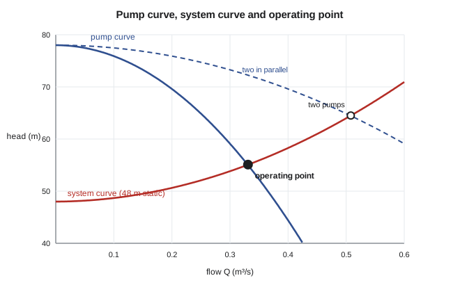
For a given piping layout, the head a pump must supply depends on the flow. From the energy equation between the source and destination surfaces, the required head is the static lift plus the losses, and the losses grow roughly with the square of the flow. Plotting required head against flow gives the system curve. It starts at the static head when the flow is zero and rises like a parabola. Opening or closing a valve, adding a pipe or changing the reservoir levels shifts the curve.
Pump characteristic curves
A centrifugal pump at a fixed speed delivers a head that falls as the flow rises. The manufacturer tests each pump model and publishes its characteristic curves: head against flow, efficiency against flow, shaft power against flow and the net positive suction head required, all at a stated speed and impeller diameter. The head curve is often well fitted by \(H = H_0 - aQ^2\), where \(H_0\) is the shutoff head at zero flow. The efficiency curve rises to a peak, the best efficiency point (BEP), and falls on either side. Pumps should be selected to run near their BEP, typically between 80 and 110 percent of BEP flow, where efficiency is high and vibration, recirculation and bearing loads are low.
Finding the operating point
A pump connected to a system runs where its head curve crosses the system curve, because there the head the pump supplies equals the head the system requires. Graphically, that is the intersection of the two curves; numerically, we solve \(H_{\text{pump}}(Q) = H_{\text{sys}}(Q)\). Because the friction factor depends on the flow, the system curve is not exactly a parabola, and a simple root-finding method such as bisection is the safest approach. The program below does exactly that for the Northside system and the proposed pump.
# Pump operating point: intersect the pump curve with the system curve, then check NPSH
import math
rho, mu, g = 998.0, 1.0e-3, 9.81

def colebrook(Re, rel):
    x = -1.8 * math.log10(6.9 / Re + (rel / 3.7) ** 1.11)
    for _ in range(60):
        x = -2.0 * math.log10(rel / 3.7 + 2.51 * x / Re)
    return 1 / x**2

# System: clearwell (z = 0) to reservoir (z = 48 m) through suction and discharge pipes
D, L, e = 0.500, 1250.0, 0.25e-3
K_sum = 0.5 + 2 * 0.3 + 4 * 0.25 + 1.0 + 2.5    # entrance, gate valves, elbows, exit, check valve
dz = 48.0

def system_head(Q):
    if Q <= 0: return dz
    V = Q / (math.pi * D**2 / 4)
    f = colebrook(rho * V * D / mu, e / D)
    return dz + (f * L / D + K_sum) * V**2 / (2 * g)

# Pump curve from the manufacturer's test points, fitted as H = H0 - a Q^2
H0, a = 78.0, 210.0          # m, s^2/m^5
pump_head = lambda Q: H0 - a * Q**2
eta = lambda Q: 0.86 * (1 - ((Q - 0.32) / 0.32) ** 2)   # efficiency curve, best near 0.32 m3/s

lo, hi = 0.01, math.sqrt(H0 / a)
for _ in range(80):                  # bisection on pump head minus system head
    mid = (lo + hi) / 2
    if pump_head(mid) - system_head(mid) > 0: lo = mid
    else: hi = mid
Q = (lo + hi) / 2
H = pump_head(Q)
P = rho * g * Q * H / eta(Q)
print(f"Operating point: Q = {Q:.3f} m3/s ({Q*1000:.0f} L/s), H = {H:.1f} m, efficiency {eta(Q):.0%}, shaft power {P/1000:.0f} kW")

# Two identical pumps in parallel: each carries Q/2 at the same head
lo, hi = 0.01, 2 * math.sqrt(H0 / a)
for _ in range(80):
    mid = (lo + hi) / 2
    if pump_head(mid / 2) - system_head(mid) > 0: lo = mid
    else: hi = mid
Q2 = (lo + hi) / 2
print(f"Two pumps in parallel: Q = {Q2:.3f} m3/s, only {Q2/Q:.2f} times one pump")

# NPSH available at the pump inlet: clearwell surface 1.5 m above the pump inlet
patm, pv = 97.4e3, 2.34e3
z_s, hL_s = 1.5, 0.6
npsha = patm / (rho * g) + z_s - hL_s - pv / (rho * g)
print(f"NPSH available = {npsha:.1f} m (compare with the pump's NPSH required, about 6 m at this flow)")Operating point: Q = 0.331 m3/s (331 L/s), H = 55.1 m, efficiency 86%, shaft power 207 kW Two pumps in parallel: Q = 0.508 m3/s, only 1.54 times one pump NPSH available = 10.6 m (compare with the pump's NPSH required, about 6 m at this flow)
The proposed pump runs at about 0.33 m³/s against 55 m of head, very close to its best efficiency point, and needs about 207 kW of shaft power. Jun's check therefore confirms the selection. The program also shows what happens when a second identical pump runs in parallel: each pump carries half the total flow at the common head, so the combined curve is the single-pump curve stretched to double the flow. The combined flow rises only to about 0.51 m³/s, about 1.5 times one pump, because the system curve climbs steeply with flow. Parallel pumps are best suited to systems whose curve is dominated by static lift; in friction-dominated systems, adding a pump gains little.
Pumps in series, by contrast, add their heads at the same flow, which suits systems with high static lifts. Variable-speed drives offer a third option. The affinity laws say that, for a given pump, flow varies with speed, head with speed squared and power with speed cubed. Slowing a pump by 20 percent cuts its power at a similar operating point by nearly half, which is why variable-speed drives often pay for themselves quickly in systems where demand varies.
Cavitation and net positive suction head
The lowest pressure in a pump occurs at the eye of the impeller, just inside the inlet. If it falls to the vapor pressure, the pump cavitates, losing head and suffering pitting damage, as described in Lesson 1. To prevent this, the absolute head at the pump inlet must exceed the vapor pressure head by a margin the manufacturer specifies, the net positive suction head required, NPSHR. The system provides the net positive suction head available, NPSHA, which follows from the energy equation between the source surface and the pump inlet.
Here \(z_s\) is the height of the source surface above the pump inlet (negative if the pump is above the water), and \(h_{L,s}\) is the head loss in the suction piping. The design rule is \(\text{NPSH}_A > \text{NPSH}_R\) with a margin, often 1 to 1.5 m or a ratio of at least 1.1 to 1.3, depending on the pump type and the water temperature. Everything that lowers NPSHA makes cavitation more likely: high elevation, warm water, a pump set high above the water, long or restricted suction piping, and running at flows beyond the BEP, where NPSHR rises sharply.
Worked problem
NPSH available at Pump 2
The clearwell surface is 1.5 m (4.9 ft) above the pump inlet, the suction head loss is 0.6 m, the barometer reads 97.4 kPa and the water is at 20 °C (\(p_v = 2.34\ \text{kPa}\)). Find NPSHA and compare it with the NPSHR of 6.0 m (19.7 ft) at the operating flow.
Show solution
- Atmospheric pressure head: \(97.4 \times 1000/(998 \times 9.81)\) m, about 9.7 to 10.0 m.
- Vapor pressure head: \(2340/(998 \times 9.81) = 0.24\ \text{m}\).
- \(\text{NPSH}_A = p_{\text{atm}}/\gamma + 1.5 - 0.6 - 0.24\).
Answer: NPSHA is about 10.6 m (34.8 ft) against an NPSHR of 6.0 m, a comfortable margin. On a hot summer day with the clearwell drawn down 2 m, the margin would shrink to about 2 m, still acceptable, which Jun notes in his report.
Pipes in series, parallel and networks
Real systems have more than one pipe. For pipes in series, the same flow passes through each, and the head losses add. For pipes in parallel between two junctions, the head loss is the same along each path, and the flows add; the flow divides so that each branch loses the same head. Whole distribution networks, with hundreds of loops and nodes, are solved by applying continuity at every node and equal head loss around every loop. The Hardy Cross method did this by hand in the 1930s; today's network models solve the same equations by matrix methods, and Platte Bluffs Water keeps a calibrated model of its entire system to plan new mains, size pumps and check fire flows.
Jun's report closed with a summary that every hydraulic design should include: the operating point and efficiency of each pump, the system curve under minimum and maximum reservoir levels, the NPSH margin, the maximum pressures along the main from the hydraulic grade line, and the energy cost per year. With those numbers, Hana approved the pump order, and the course's tools, from the properties of water to the energy equation, had produced a decision worth several hundred thousand dollars over the pump's life.
Common mistakes
MistakeIgnoring the exit loss into a reservoir.
InsteadThe exit loss is a full velocity head, K = 1.
MistakeUsing the larger pipe's velocity with K for a contraction or enlargement.
InsteadUse the velocity the coefficient is defined with, usually the smaller pipe's.
MistakeAssuming two parallel pumps double the flow.
InsteadThey double the flow at a given head, but the system curve rises, so the gain is smaller.
MistakeComputing NPSH with gauge pressure.
InsteadNPSH uses absolute pressure: atmospheric pressure head minus vapor pressure head.
MistakeSelecting a pump whose operating point is far from its BEP.
InsteadAim for roughly 80–110 % of BEP flow for efficiency and reliability.
Summary and key terms
- Minor losses are h_m = KV²/(2g); total loss h_L = (fL/D + ΣK)V²/(2g).
- The exit loss into a reservoir is one velocity head; a rounded entrance nearly eliminates entrance loss.
- The system curve is static head plus losses, rising roughly as Q².
- A pump operates where its head curve crosses the system curve.
- Parallel pumps add flow at equal head; series pumps add head at equal flow.
- Affinity laws: Q ∝ N, H ∝ N², P ∝ N³.
- Cavitation is avoided when NPSHA = p_atm/γ + z_s − h_L,s − p_v/γ exceeds NPSHR with a margin.
- Minor loss
- Head loss caused by a fitting, valve, entrance, exit or change of section.
- Loss coefficient
- The factor K relating a minor loss to the velocity head.
- Equivalent length
- The length of straight pipe with the same loss as a fitting, KD/f.
- System curve
- The head required by a piping system plotted against flow.
- Pump curve
- The head a pump delivers plotted against flow at a fixed speed.
- Operating point
- The flow and head where the pump curve and system curve intersect.
- Best efficiency point
- The flow at which a pump's efficiency is highest.
- Shutoff head
- The head a centrifugal pump develops at zero flow.
- Affinity laws
- Scaling rules relating flow, head and power to pump speed.
- NPSH available
- The absolute head above vapor pressure at the pump inlet provided by the system.
- NPSH required
- The minimum NPSH a pump needs to avoid harmful cavitation, from the manufacturer.
Practice problems
Work each problem on paper first, then reveal the answer to check.
Find the loss through a fully open globe valve (K = 8) in a 150 mm line carrying 30 L/s.
Show answer
V = 1.70 m/s; h = 8(1.70²/19.62) = 1.18 m.
Water flows from a 100 mm pipe into a 200 mm pipe at 2 m/s in the smaller pipe. Find the enlargement loss.
Show answer
K = (1 − 0.25)² = 0.5625; h = 0.5625(2²/19.62) = 0.115 m.
A system has 30 m of static lift and 12 m of loss at 0.20 m³/s. Write its approximate system curve.
Show answer
H = 30 + 300Q² (Q in m³/s, H in m).
A pump curve is H = 60 − 400Q². Find the operating point with the system in the previous question.
Show answer
60 − 400Q² = 30 + 300Q², so Q = 0.207 m³/s and H = 42.9 m.
A pump running at 1780 rpm delivers 0.30 m³/s at 55 m and 195 kW. Estimate its flow, head and power at 1500 rpm.
Show answer
Q = 0.253 m³/s, H = 39.1 m, P = 117 kW.
In the program, raise the static lift to 52 m. What happens to the flow?
Show answer
It falls to about 0.31 m³/s at 58 m, because the system curve shifts up.
Lesson quiz · 5 questions
Score 60% or more to complete this lesson.
Create a free account to save your progress, take quizzes and earn a certificate.