
STAT-235 · Lesson 5 of 5 · 28 min
Linear regression
Much of engineering is about relationships between variables: concrete strength and water–cement ratio, sensor voltage and applied load, fuel consumption and speed, pavement deterioration and traffic. Regression finds the equation that best describes such a relationship from data, measures how well it fits, and, crucially, says how uncertain predictions made from it are. It is the statistical tool engineers use most, from calibrating instruments to building the empirical equations found throughout design codes.
This chapter covers scatter plots and correlation, least-squares fitting, residuals and R², inference about the slope, confidence and prediction intervals, and the traps: extrapolation, outliers, and mistaking correlation for causation.
Scatter plots and correlation
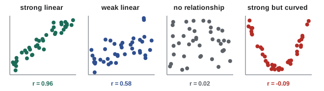
Always start with a scatter plot. It shows the form of the relationship (straight or curved), its direction, its strength, and any unusual points, none of which a single number can capture. The correlation coefficient r summarizes the strength of a straight-line relationship:
r lies between −1 and +1. Values near ±1 mean the points cluster tightly about a line; values near 0 mean no linear relationship. The sign gives the direction. r measures only linear association: a perfect U-shaped relationship can have r = 0.
Fitting a line by least squares
The simple linear regression model is
where ε is random scatter about the line, assumed independent with mean 0 and constant standard deviation σ. The least-squares line chooses the intercept \(b_0\) and slope \(b_1\) that minimize the sum of squared vertical distances (residuals) from the points to the line. Setting the partial derivatives to zero, the same optimization as MATH-209, gives
The line always passes through the point \((\bar{x}, \bar{y})\). The slope is the estimated change in y per unit change in x.
Worked problem
Strength and water–cement ratio
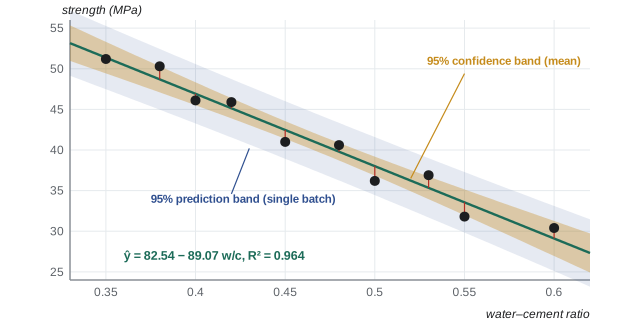
Ten trial batches gave these water–cement ratios w and 28-day strengths y (MPa): (0.35, 51.2), (0.38, 50.3), (0.40, 46.1), (0.42, 45.9), (0.45, 41.0), (0.48, 40.6), (0.50, 36.2), (0.53, 36.9), (0.55, 31.8), (0.60, 30.4). Fit a least-squares line and find r.
Show solution
- \(\bar{w} = 0.466\), \(\bar{y} = 41.04\); \(S_{ww} = 0.05804\), \(S_{wy} = -5.1694\), \(S_{yy} = 477.54\).
- \(b_1 = -5.1694/0.05804 = -89.07\) MPa per unit w/c.
- \(b_0 = 41.04 - (-89.07)(0.466) = 82.54\) MPa.
- \(r = -5.1694/\sqrt{0.05804 \times 477.54} = -0.982\).
Answer: \(\hat{y} = 82.54 - 89.07w\), r = −0.982. Each 0.01 increase in w/c lowers strength by about 0.89 MPa, the familiar rule that extra water weakens concrete
Residuals and goodness of fit
A residual is the vertical distance from a point to the line, \(e_i = y_i - \hat{y}_i\). The residual standard deviation estimates σ, the typical scatter about the line:
Two parameters were estimated, so the divisor is n − 2. The coefficient of determination \(R^2\) is the fraction of the variation in y explained by the line:
For the concrete data, the residual sum of squares is 17.13, so \(s_e = \sqrt{17.13/8} = 1.46\) MPa and \(R^2 = 1 - 17.13/477.54 = 0.964\): the water–cement ratio explains 96% of the variation in strength among these batches, and the remaining scatter is about ±1.5 MPa.
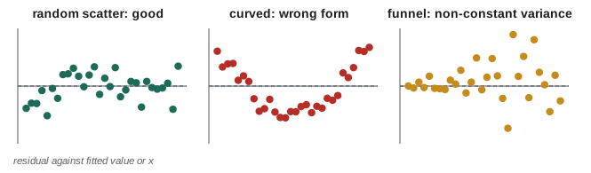
A high R² does not by itself mean the model is right. The residual plot (residuals against x or against fitted values) is the key diagnostic. Residuals should look like random scatter in a horizontal band. A curved pattern means a straight line is the wrong form; a funnel shape means the scatter grows with x (non-constant variance); a single huge residual flags an outlier to investigate.
Inference about the slope
The slope estimate varies from sample to sample, with standard error
A confidence interval is \(b_1 \pm t_{\alpha/2,\,n-2}\,SE(b_1)\), and the test of H₀: β₁ = 0 (no linear relationship) uses \(t = b_1/SE(b_1)\) with n − 2 degrees of freedom.
Worked problem
How precisely is the slope known?
For the concrete data, find a 95% confidence interval for the slope and test whether the relationship is significant.
Show solution
- \(SE(b_1) = 1.463/\sqrt{0.05804} = 6.07\).
- \(t_{0.025,8} = 2.306\): \(-89.07 \pm 2.306(6.07) = (-103.1,\ -75.1)\).
- \(t = -89.07/6.07 = -14.7\); p < 0.0001.
Answer: Slope between −103 and −75 MPa per unit w/c; overwhelming evidence of a relationship. The interval, not the p-value, tells a mix designer how much the strength–water rule could vary
Predicting: confidence and prediction intervals
At a chosen value \(x_0\), the line gives \(\hat{y}_0 = b_0 + b_1x_0\). Two different intervals answer two different questions:
- Confidence interval for the mean response: where is the average y of all batches at \(x_0\)?
- Prediction interval for one new observation: where will the next single batch fall?
The extra 1 under the root is the scatter of an individual about the mean, so prediction intervals are always wider, and they do not shrink to zero however much data you collect. Both widen as \(x_0\) moves away from \(\bar{x}\): the model is best known near the middle of the data.
Worked problem
Designing a mix
At w/c = 0.45, give a 95% confidence interval for mean strength and a 95% prediction interval for a single batch. Then find the w/c at which a single batch is 95% sure (one-sided) to reach at least 40 MPa.
Show solution
- \(\hat{y} = 82.54 - 89.07(0.45) = 42.47\) MPa.
- Mean: \(42.47 \pm 2.306(1.463)\sqrt{0.1 + (0.016)^2/0.05804} = 42.47 \pm 1.09\) MPa.
- Single batch: \(42.47 \pm 2.306(1.463)\sqrt{1.1 + 0.0044} = 42.47 \pm 3.55\) MPa.
- For a one-sided 95% lower prediction bound, use \(t_{0.05,8} = 1.860\) and search over w/c: at w/c = 0.445 the bound is 40.05 MPa; at 0.45 it is 39.61 MPa.
Answer: Mean 41.4 to 43.6 MPa; single batch 38.9 to 46.0 MPa. To be 95% sure a batch reaches 40 MPa, specify w/c ≤ 0.445, not the 0.478 where the line itself crosses 40 MPa. Designing to the line would give a weak batch about half the time
Extrapolation, outliers and causation
A regression is only trustworthy within the range of the data. The concrete line predicts 60 MPa at w/c = 0.25 and 11 MPa at 0.80, but the real relationship is curved (strength falls roughly exponentially with w/c, Abrams' law), very low ratios cannot be compacted properly, and no data were taken there. Extrapolation is the most common misuse of regression in practice.
Influential points, observations far from the others in x, can pull the line strongly toward themselves. Check them: a data-entry error should be corrected; a genuine unusual point should be reported, and the model fitted with and without it.
Finally, correlation is not causation. Across Canadian cities, the number of fire trucks dispatched correlates with fire damage, but sending trucks does not cause damage; bigger fires cause both. A third variable (a lurking or confounding variable) can create a correlation between two variables that do not affect each other. Only a designed experiment, in which x is deliberately set and other factors are controlled or randomized, as in the trial batches above, supports a causal conclusion directly.
Calibration and multiple regression
Calibrating an instrument is regression in reverse. Known inputs (reference loads) are applied, the outputs (voltages) recorded and a line fitted; in use, an output reading is converted back to the input by solving the line for x. A load cell giving 0.02, 1.03, 2.05, 2.98, 4.01 and 5.03 V at 0, 10, 20, 30, 40 and 50 kN fits \(V = 0.0257 + 0.09977L\), so a reading of 3.50 V means \(L = (3.50 - 0.0257)/0.09977 = 34.8\) kN.
Real responses usually depend on several variables. Multiple regression fits \(y = \beta_0 + \beta_1x_1 + \beta_2x_2 + \cdots\) by the same least-squares principle, solved with matrices (MATH-125): for example, strength as a function of w/c, cement content and curing temperature, or energy use of a building as a function of outdoor temperature and occupancy. Each coefficient estimates the effect of its variable with the others held fixed. Software reports each coefficient with its standard error, and the same cautions about residual plots, extrapolation and causation apply.
import numpy as np
from scipy import stats

wc = np.array([0.35, 0.38, 0.40, 0.42, 0.45, 0.48, 0.50, 0.53, 0.55, 0.60])
fc = np.array([51.2, 50.3, 46.1, 45.9, 41.0, 40.6, 36.2, 36.9, 31.8, 30.4])

fit = stats.linregress(wc, fc)
print(f"strength = {fit.intercept:.2f} + ({fit.slope:.2f}) w/c")
print(f"r = {fit.rvalue:.3f}, R^2 = {fit.rvalue**2:.3f}, SE(slope) = {fit.stderr:.2f}")

# 95% prediction interval for one batch at w/c = 0.45
n = len(wc)
resid = fc - (fit.intercept + fit.slope * wc)
se = np.sqrt(np.sum(resid**2) / (n - 2))
x0 = 0.45
y0 = fit.intercept + fit.slope * x0
half = stats.t.ppf(0.975, n - 2) * se * np.sqrt(1 + 1/n + (x0 - wc.mean())**2 / np.sum((wc - wc.mean())**2))
print(f"At w/c = {x0}: {y0:.2f} MPa, 95% PI {y0 - half:.1f} to {y0 + half:.1f} MPa")
Output: strength = 82.54 + (-89.07) w/c; r = -0.982, R^2 = 0.964, SE(slope) = 6.07; At w/c = 0.45: 42.47 MPa, 95% PI 38.9 to 46.0 MPa.
Common mistakes
MistakeFitting a line without looking at a scatter plot.
InsteadPlot first; a straight line may be the wrong form, or one point may dominate.
MistakeReading a high R² as proof that the model is correct.
InsteadCheck the residual plot for curvature, funnels and outliers.
MistakeUsing the confidence interval for the mean to predict a single new value.
InsteadUse the wider prediction interval for individual observations.
MistakeExtrapolating beyond the range of the data.
InsteadPredictions are only supported within the observed x range.
MistakeConcluding that x causes y from observational data.
InsteadLook for lurking variables; causal claims need designed experiments.
MistakeDesigning to the fitted line.
InsteadHalf the outcomes fall below the line; design to a prediction bound.
Summary and key terms
- Start with a scatter plot; r measures the strength and direction of linear association only.
- Least squares: b₁ = Sxy/Sxx, b₀ = ȳ − b₁x̄; the line passes through (x̄, ȳ).
- Residuals e = y − ŷ; s_e = √(Σe²/(n − 2)); R² = 1 − Σe²/Syy is the fraction of variation explained.
- Residual plots reveal wrong form, non-constant variance and outliers.
- Slope inference: SE(b₁) = s_e/√Sxx with n − 2 degrees of freedom.
- Prediction intervals for single values are wider than confidence intervals for the mean; both widen away from x̄. Avoid extrapolation, and do not infer causation from correlation alone.
- Scatter plot
- A plot of paired (x, y) data points.
- Correlation coefficient
- r, a measure from −1 to 1 of the strength of linear association.
- Least squares
- Choosing parameters to minimize the sum of squared residuals.
- Residual
- The observed value minus the fitted value.
- Coefficient of determination
- R², the fraction of variation in y explained by the model.
- Residual standard deviation
- s_e, the typical scatter of points about the fitted line.
- Prediction interval
- An interval for a single future observation at a given x.
- Extrapolation
- Using a model outside the range of the data used to fit it.
- Influential point
- An observation that strongly changes the fitted line.
- Lurking variable
- An unmeasured variable that affects both x and y, creating a misleading correlation.
- Calibration
- Fitting the relationship between an instrument's output and known inputs.
- Multiple regression
- Regression of y on several predictor variables at once.
Practice problems
Work each problem on paper first, then reveal the answer to check.
For n = 5 points, x̄ = 4, ȳ = 10, Sxx = 20, Sxy = 50, Syy = 140. Find the least-squares line and r.
Show answer
b₁ = 2.5; b₀ = 10 − 2.5 × 4 = 0; ŷ = 2.5x; r = 50/√(20 × 140) = 0.945.
For the previous problem, find R² and the residual sum of squares.
Show answer
R² = 0.893; SSE = (1 − 0.893) × 140 = 15.0 (equivalently Syy − Sxy²/Sxx = 140 − 125 = 15).
A regression of fuel use (L/100 km) on vehicle mass (t) gives ŷ = 2.1 + 4.8x. Interpret the slope and predict fuel use for a 1.5 t vehicle.
Show answer
Each extra tonne adds about 4.8 L/100 km; ŷ = 2.1 + 7.2 = 9.3 L/100 km.
The data in the previous problem covered vehicles from 1.0 to 2.5 t. Should the model be used for a 15 t truck?
Show answer
No: that is far outside the data range (extrapolation), and trucks differ in many other ways.
A residual plot shows residuals that increase in spread as x increases. What does this indicate?
Show answer
Non-constant variance; consider transforming y (for example ln y) or weighted least squares.
With b₁ = 3.2, SE(b₁) = 1.1 and n = 12, is the slope significant at α = 0.05 (t₀.₀₂₅,₁₀ = 2.228)?
Show answer
t = 2.91 > 2.228: yes. 95% CI: 3.2 ± 2.45 = (0.75, 5.65).
Explain why the prediction interval at x̄ is wider than the confidence interval at x̄.
Show answer
It includes the scatter of an individual observation about the mean (the extra 1 under the square root), not just the uncertainty in the line.
Across cities, ice-cream sales correlate with the number of drownings. Give a lurking variable.
Show answer
Hot weather: it increases both ice-cream sales and swimming.
A thermocouple calibration gives V = 0.10 + 0.041T (mV, °C). What temperature corresponds to 4.20 mV?
Show answer
T = (4.20 − 0.10)/0.041 = 100 °C.
Data appear to follow y = ae^{bx}. How can linear regression be used to estimate a and b?
Show answer
Regress ln y on x: the slope is b and the intercept is ln a, so a = e^(intercept).
Lesson quiz · 5 questions
Score 60% or more to complete this lesson.
Create a free account to save your progress, take quizzes and earn a certificate.