
ROB-360 · Lesson 8 of 12 · 29 min
Hardware-in-the-loop testing and sim-to-real transfer
Every simulation is wrong somewhere. Masses are slightly off, friction varies from floor to floor, motors saturate, cameras see glare, latencies differ, and people do things no scenario writer imagined. The difference between how software behaves in simulation and how it behaves on the real robot is called the reality gap. This lesson covers the techniques that narrow the gap and that test the parts simulation cannot: system identification to calibrate models, domain randomization to make software robust to what remains, hardware-in-the-loop testing that puts real controllers and sensors into the loop, metrics that measure the gap, and the staged path from simulation to field.
Where the reality gap comes from
The gap has many sources. Model parameters may be wrong: mass, inertia, friction, motor constants, sensor noise. Some physics may be missing entirely: cable drag on an arm, tyre deformation, airflow, thermal effects on sensors. Timing usually differs, because simulated sensors arrive on time and in order while real ones jitter, and real computers have competing loads. Perception sees different data, since rendered images lack the lens flare, motion blur, dust and lighting variety of real cameras. And the environment differs, with clutter, reflective surfaces and human behaviour that worlds rarely capture. Some gaps can be closed by better modelling; others are cheaper to cover with robustness and real testing.
| Source of gap | Example | Typical remedy |
|---|---|---|
| Wrong parameters | Robot mass 10 % low, wheel friction too high | System identification from real data |
| Missing physics | Cable drag, tyre deformation, backlash | Add models where tests show they matter |
| Timing and latency | Camera frames arrive 40 ms late with jitter | Simulate delays and jitter; hardware-in-the-loop |
| Perception realism | Glare, blur, unusual materials | Real data replay, domain randomization, photorealistic rendering |
| Environment and people | Clutter, unexpected human behaviour | Scenario libraries from field logs; field tests |
System identification
System identification estimates model parameters from measured input and output data. For a robot drive, a simple experiment applies a step in commanded velocity and records the actual wheel speed; fitting a first-order model gives the time constant and gain. For an arm, exciting trajectories and joint torque measurements can identify inertial and friction parameters, often with least-squares methods in which the dynamics are written linearly in the unknown parameters (ROB-300). The identified parameters then replace guesses in the simulation model, and the same data is kept as a validation set: after updating the model, simulate the same commands and compare.
import math, random
# Identify a first-order wheel-speed response  w(t) = K u (1 - exp(-t/tau)) from noisy step data
rnd = random.Random(3)
K_true, tau_true, u = 0.95, 0.18, 1.0                # gain and time constant (s)
ts = [i * 0.01 for i in range(1, 101)]
meas = [K_true * u * (1 - math.exp(-t / tau_true)) + rnd.gauss(0, 0.01) for t in ts]
# Steady state gives K; then fit tau by least squares on ln(1 - w / (K u))
K_est = sum(meas[-20:]) / 20 / u
num = den = 0.0
for t, w in zip(ts, meas):
    r = 1 - w / (K_est * u)
    if 0.05 < r < 0.95:                              # use the informative part of the curve
        y = math.log(r)                              # y = -t / tau
        num += t * y; den += t * t
tau_est = -den / num
print(f"identified K = {K_est:.3f} (true {K_true}), tau = {tau_est:.3f} s (true {tau_true})")
print(f"default model guess tau = 0.05 s would be off by a factor of {tau_true / 0.05:.1f}")identified K = 0.943 (true 0.95), tau = 0.182 s (true 0.18) default model guess tau = 0.05 s would be off by a factor of 3.6
Worked problem
What the time constant changes
A simulation assumes the drive reaches commanded speed almost instantly (time constant 0.05 s), but identification gives 0.18 s. A planner commands a stop from 1.0 m/s when an obstacle is detected. How much extra distance does the real robot cover during the lag, approximating the extra distance as speed times the difference in time constants?
Show solution
- For a first-order lag, the distance covered beyond an ideal instant stop is about \( v \tau \).
- Simulation: \( 1.0 \times 0.05 = 0.05 \) m. Real: \( 1.0 \times 0.18 = 0.18 \) m.
- Extra: about 0.13 m, which the safety margin must cover.
Answer: About 13 cm more stopping distance than the simulation predicts. Uncalibrated dynamics make simulated safety tests optimistic.
Domain randomization
Even a calibrated model is never exact, and real conditions vary from robot to robot and day to day. Domain randomization deliberately varies simulation parameters across runs (masses, friction, sensor noise, latencies, lighting, textures, object positions) so that software or learned policies that work across the whole range are more likely to work on the real robot, which becomes just one more sample from the range. The idea became famous in robot learning, where policies trained only in randomized simulation transferred to real hardware, but it is equally useful for testing conventional software: a navigation stack that succeeds across a thousand randomized worlds is more trustworthy than one that succeeds in one perfect world.
Ranges must be chosen with care. Too narrow and the real robot falls outside them; too wide and the tests demand robustness that is unnecessary or impossible, or learned policies become overly cautious. Identified parameters with their uncertainty are a good starting point: centre the range on the identified value and make it a few standard deviations wide, and widen it for parameters known to vary in the field, such as floor friction.
import random
rnd = random.Random(360)
# Sample randomized scenario parameters around identified values (ranges illustrative)
ranges = {"mass_kg": (38.0, 46.0), "wheel_mu": (0.35, 0.9), "tau_s": (0.14, 0.24),
          "lidar_sigma_m": (0.008, 0.03), "cam_latency_ms": (25, 90), "light_lux": (80, 2000)}
def sample():
    p = {k: rnd.uniform(*v) for k, v in ranges.items()}
    p["floor"] = rnd.choice(["sealed concrete", "painted concrete", "epoxy, wet patch"])
    return p
runs = [sample() for _ in range(1000)]
for k in ("wheel_mu", "cam_latency_ms"):
    vals = sorted(r[k] for r in runs)
    print(f"{k:14} min {vals[0]:7.3f}  median {vals[500]:7.3f}  max {vals[-1]:7.3f}")
wet = sum(r["floor"] == "epoxy, wet patch" for r in runs)
print(f"runs with a wet patch: {wet} of {len(runs)}")
print("example run:", {k: (round(v, 3) if isinstance(v, float) else v) for k, v in runs[0].items()})wheel_mu min 0.350 median 0.613 max 0.900
cam_latency_ms min 25.054 median 59.253 max 89.877
runs with a wet patch: 360 of 1000
example run: {'mass_kg': 45.359, 'wheel_mu': 0.519, 'tau_s': 0.232, 'lidar_sigma_m': 0.01, 'cam_latency_ms': 38.466, 'light_lux': 358.225, 'floor': 'sealed concrete'}Hardware-in-the-loop testing
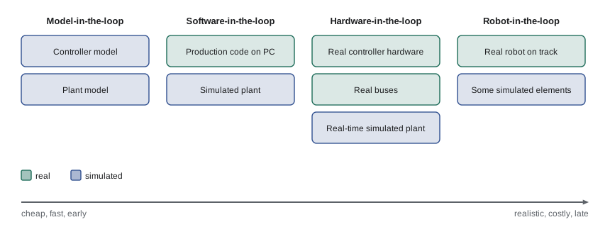
Hardware-in-the-loop (HIL) testing connects real hardware to a simulated environment. In the most common form, the real controller, such as a motor drive, an embedded flight controller or the robot's main computer, runs its real software and talks over its real interfaces (CAN, EtherCAT, serial) to a real-time simulator that pretends to be the rest of the robot and the world. HIL tests catch problems that software-only simulation hides: timing on the real processor, interrupt latency, bus load and message timing, numerical differences on embedded hardware, firmware bugs and configuration mistakes. Related terms describe how much is real: software-in-the-loop (SIL) runs production code on a development computer against a simulation; processor-in-the-loop runs it on the target processor; vehicle- or robot-in-the-loop runs the full robot on a test stand or track with simulated elements such as virtual obstacles.
Worked problem
Can the HIL simulator keep up?
A HIL rig simulates a robot joint for a real motor controller that runs a 10 kHz current loop and a 1 kHz position loop over EtherCAT. The simulator computes the joint model in 35 µs and needs 20 µs for I/O each cycle. Can it close the loop at 10 kHz?
Show solution
- Cycle time at 10 kHz: 100 µs.
- Simulator work per cycle: \( 35 + 20 = 55 \) µs, which is 55 % of the cycle.
- The remaining 45 µs must absorb jitter; the simulator must run on a real-time operating system so worst-case times, not averages, stay under 100 µs (ROB-320).
Answer: Yes, with 45 µs of margin, provided worst-case timing is guaranteed by a real-time platform. If the model grew to 90 µs, the rig would need a faster computer, an FPGA or a simpler model.
Measuring the reality gap
A reality gap should be measured, not argued about. The usual method is to run matched experiments in simulation and on the real robot, with the same commands, routes or scenarios, and compare the outcomes with chosen metrics: tracking error, stopping distance, path length, time to goal, success rate, localization error or perception precision and recall. Because both sides are random, distributions are compared rather than single runs. Simple statistics such as differences in means with confidence intervals, or distribution distances such as the Kolmogorov–Smirnov statistic (the largest gap between two cumulative distributions), make the comparison objective and trackable over time.
import random
rnd = random.Random(11)
# Stopping distances (m) from 40 real trials and 400 simulated trials at 1.0 m/s
real = [rnd.gauss(0.62, 0.05) for _ in range(40)]
sim_before = [rnd.gauss(0.49, 0.03) for _ in range(400)]    # before identification
sim_after = [rnd.gauss(0.61, 0.045) for _ in range(400)]    # after identification + randomization
def ks(a, b):                                               # Kolmogorov-Smirnov statistic
    pts = sorted(a + b)
    return max(abs(sum(x <= p for x in a) / len(a) - sum(x <= p for x in b) / len(b)) for p in pts)
mean = lambda xs: sum(xs) / len(xs)
for name, sim in (("before", sim_before), ("after", sim_after)):
print(f"{name}: mean gap {mean(real) - mean(sim):+.3f} m, KS = {ks(real, sim):.2f}")before: mean gap +0.130 m, KS = 0.94 after: mean gap +0.012 m, KS = 0.17
With 40 real samples, a KS statistic above roughly 0.22 indicates a significant difference at the 5 % level. Here the uncalibrated simulation is clearly different from reality, while the calibrated one is not distinguishable with this much data. Teams set acceptance thresholds for such metrics and recheck them whenever the robot hardware or simulator changes, so the evidence that simulation can be trusted for a given test stays current.
From simulation to the field
A staged path keeps risk low and evidence growing. New software passes unit and integration tests, then the simulation suite, then HIL or test-stand checks for anything touching real-time control or hardware interfaces, then a test track or mock-up of the customer site, then supervised trials at a pilot site, and finally gradual deployment with monitoring. Each stage has entry and exit criteria tied to requirements. Field logs flow back into the earlier stages: every interesting failure in the field becomes a regression scenario in simulation or a golden replay bag (lesson 4), so the simulation suite steadily absorbs the real world's surprises.
Worked problem
Allocating test hours
A release needs evidence for a docking requirement of at least 99 % success. Simulation runs cost about 3 minutes each, test-track trials 15 minutes each with staff, and the team has 20 staff-hours of track time. How many track trials are possible, and what is simulation's role?
Show solution
- Track trials: \( 20 \times 60 / 15 = 80 \).
- Eighty successes alone support a failure rate below only about \( 3/80 \approx 3.8 \) % (lesson 2).
- Simulation can run thousands of docking attempts overnight, provided the reality gap for docking has been measured and is small.
Answer: About 80 track trials, not enough on their own to show 99 %. The usual argument combines a validated simulation with thousands of runs and a smaller set of real trials that confirm the simulation's fidelity.
Common mistakes
MistakeTreating a simulated pass as proof that the real robot works
InsteadMeasure the reality gap for the metrics that matter and keep real tests in the plan.
MistakeGuessing actuator and friction parameters
InsteadIdentify them from real experiments and keep validation data.
MistakeRandomizing parameters over arbitrary, very wide ranges
InsteadCentre ranges on identified values with realistic spread.
MistakeTesting real-time controllers only in software simulation
InsteadUse hardware-in-the-loop to test timing, buses and firmware.
MistakeComparing one real run against one simulated run
InsteadCompare distributions with statistics such as mean differences and the KS statistic.
Summary and key terms
- The reality gap comes from wrong parameters, missing physics, timing, perception realism and the environment.
- System identification estimates model parameters from real data, and the data also validates the updated model.
- Domain randomization varies parameters across runs so software is robust to the remaining gap.
- Hardware-in-the-loop testing puts real controllers and interfaces in the loop with a real-time simulation.
- MIL, SIL, HIL and robot-in-the-loop form a ladder from cheap and early to realistic and late.
- The gap should be measured with matched experiments and distribution statistics against thresholds.
- A staged path from simulation to field, with field failures fed back as scenarios, builds evidence safely.
- Reality gap
- The difference between behaviour in simulation and on the real robot.
- System identification
- Estimating model parameters from measured input and output data.
- Time constant
- For a first-order system, the time to reach about 63 % of a step change.
- Domain randomization
- Varying simulation parameters across runs to build robustness.
- Hardware-in-the-loop
- Testing real hardware against a real-time simulated environment.
- Software-in-the-loop
- Running production code on a development computer against a simulation.
- Validation data
- Measurements held back to check a model after it is updated.
- Kolmogorov–Smirnov statistic
- The largest gap between two cumulative distributions.
- Matched experiment
- The same commands or scenario run in simulation and on the real robot.
- Entry and exit criteria
- Conditions for starting and finishing a test stage.
Practice problems
Work each problem on paper first, then reveal the answer to check.
Name three sources of the reality gap.
Show answer
For example wrong parameters, timing differences and perception realism.
What experiment identifies a drive's time constant?
Show answer
A step in commanded speed with the response recorded.
Why keep validation data after identification?
Show answer
To check that the updated model matches data it was not fitted to.
What is domain randomization?
Show answer
Varying simulation parameters across runs to make software robust.
How should randomization ranges be chosen?
Show answer
Centred on identified values with realistic spread, wider for parameters that vary in the field.
What does HIL catch that SIL misses?
Show answer
Real processor timing, bus behaviour and firmware issues.
A HIL cycle is 200 µs and the simulator needs 150 µs. What is the margin?
Show answer
50 µs, which must cover worst-case jitter.
What does the KS statistic measure?
Show answer
The largest gap between two cumulative distributions.
Why compare distributions instead of single runs?
Show answer
Both simulation and reality are random.
What should happen to field failures?
Show answer
They should become regression scenarios or replay tests.
Lesson quiz · 5 questions
Score 60% or more to complete this lesson.
Create a free account to save your progress, take quizzes and earn a certificate.