Scattering theory: the Lippmann–Schwinger equation, the Born series and the optical theorem

Scattering experiments are how physics learns about forces it cannot see directly, from Rutherford's discovery of the nucleus to the measurement of quark structure and the search for dark matter. PHYS-373 treated scattering by the method of partial waves and by the first Born approximation. This lesson rebuilds the theory from a single exact equation, the Lippmann–Schwinger equation, of which the Born approximation is the first step of an iteration. The same framework leads to the optical theorem, a general relation between the forward scattering amplitude and the total cross-section that follows from conservation of probability alone.

The scattering problem

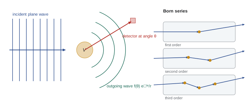
A particle of mass \(m\) and energy \(E = \hbar^2k^2/2m > 0\) approaches a potential \(V(\mathbf r)\) that vanishes outside a finite region, or falls off faster than \(1/r\). Far from the target the stationary state is an incident plane wave plus an outgoing spherical wave,

and the scattering amplitude \(f\) determines everything measurable. The differential cross-section is \(d\sigma/d\Omega = |f|^2\), the number of particles scattered per unit solid angle divided by the incident flux, and the total cross-section is its integral over all directions. The task of scattering theory is to compute \(f\) from \(V\), or, in the inverse problem, to infer \(V\) from measured cross-sections.

The Lippmann–Schwinger equation

Write the time-independent Schrödinger equation as \((\nabla^2 + k^2)\psi = U\psi\), with \(U = 2mV/\hbar^2\). The free equation \((\nabla^2 + k^2)\phi = 0\) has plane-wave solutions. The full equation can be converted into an integral equation with the Green's function of the free operator, the solution of \((\nabla^2 + k^2)G = \delta^3(\mathbf r)\). Of the possible solutions, the one with outgoing waves is

Then the scattering state obeys

This is the Lippmann–Schwinger equation, published by Bernard Lippmann and Julian Schwinger in 1950. It is exactly equivalent to the Schrödinger equation together with the outgoing boundary condition, which is built into \(G_+\). In operator form it reads \(|\psi^+\rangle = |\mathbf k\rangle + G_0^+V|\psi^+\rangle\) with \(G_0^+ = (E - H_0 + i\epsilon)^{-1}\). The small positive \(i\epsilon\) selects outgoing waves, a choice that reflects causality: the scattered wave appears after the incident wave arrives.

For \(r\) much larger than the range of the potential, \(|\mathbf r - \mathbf r'| \approx r - \hat{\mathbf r}\cdot\mathbf r'\). Substituting into the Green's function and comparing with the asymptotic form gives an exact formula for the amplitude:

where \(\mathbf k' = k\hat{\mathbf r}\) is the outgoing wave vector. The amplitude is a matrix element of the potential between the final plane wave and the exact scattering state. It is natural to define the transition operator \(T\) by \(V|\psi^+\rangle = T|\mathbf k\rangle\), so that \(f = -(m/2\pi\hbar^2)\langle\mathbf k'|T|\mathbf k\rangle\).

The Born series

Iterating the Lippmann–Schwinger equation, substituting \(\psi\) on the right by the whole right-hand side, gives the Born series:

Its first term is the first Born approximation of PHYS-373,

the Fourier transform of the potential at the momentum transfer \(\mathbf q\), with \(q = 2k\sin(\theta/2)\). Each later term adds one more scattering inside the potential, with free propagation between scatterings. The series is the scattering counterpart of the Dyson series of lesson 3, and the two are closely related. In field theory the Born terms become Feynman diagrams with one, two and more exchanges.

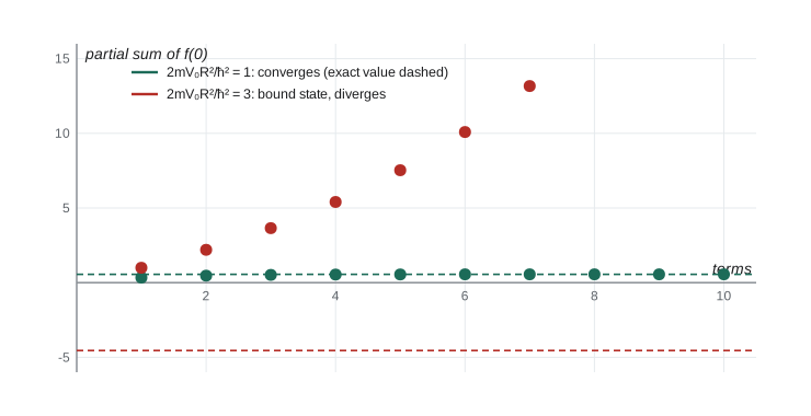
When does the series converge? Roughly, when the potential is too weak to bind a state. For an attractive square well of depth \(V_0\) and radius \(R\), at low energy the expansion parameter is \(2mV_0R^2/\hbar^2\), and the series converges for \(\sqrt{2mV_0/\hbar^2}\,R < \pi/2\), exactly the condition that the well has no bound state. At high energy the Born series converges for any potential because the particle spends little time inside it, so the first Born approximation becomes reliable at energies much larger than the depth of the well. This is why the Born approximation works well for fast electrons scattered by atoms and nuclei, and why it fails for slow neutrons on nuclei.

The optical theorem

Probability is conserved in scattering, and this has a striking consequence. The scattered wave removes particles from the forward beam, so the forward-going part of the wave must interfere destructively with the incident wave by exactly the amount that is scattered. Working this out gives the optical theorem:

The forward amplitude knows about the scattering in every direction. The theorem holds for any potential and also when particles are absorbed, provided \(\sigma_{\text{tot}}\) includes absorption, and it carries over to relativistic scattering, where it ties total cross-sections to forward amplitudes measured at colliders. It is the scattering form of unitarity, \(S^\dagger S = 1\) for the scattering operator \(S = 1 - 2\pi iT\delta(E_f - E_i)\).

In partial waves the theorem is easy to check. With \(f = (1/k)\sum_\ell(2\ell + 1)e^{i\delta_\ell}\sin\delta_\ell\,P_\ell(\cos\theta)\) and \(P_\ell(1) = 1\),

The first Born approximation violates it. For a real potential \(f^{(1)}\) is real, so \(\operatorname{Im}f^{(1)}(0) = 0\) while \(\sigma^{(1)} = \int|f^{(1)}|^2d\Omega > 0\). The imaginary part first appears at second order, \(\operatorname{Im}f^{(2)}(0) = (k/4\pi)\sigma^{(1)}\), consistent order by order. The violation is a reminder that the first Born approximation is accurate only to first order in \(V\), while the cross-section is a second-order quantity.

import cmath, math
# Units: hbar^2/2m = 1, so E = k^2 and the potential is V(r) = -V0 for r < R = 1.

def jn(l, x):
    """Spherical Bessel j_l and n_l by upward recurrence (fine for the small l used here)."""
    j = [math.sin(x) / x, math.sin(x) / x ** 2 - math.cos(x) / x]
    n = [-math.cos(x) / x, -math.cos(x) / x ** 2 - math.sin(x) / x]
    for k in range(1, l):
        j.append((2 * k + 1) / x * j[k] - j[k - 1]); n.append((2 * k + 1) / x * n[k] - n[k - 1])
    return j[l], n[l]
def djn(l, x):
    j, n = jn(l, x)
    if l == 0: return -jn(1, x)[0], -jn(1, x)[1]
    jm, nm = jn(l - 1, x)
    return jm - (l + 1) / x * j, nm - (l + 1) / x * n

def delta(l, k, V0, R=1.0):
    K = math.sqrt(k * k + V0)
    jK, _ = jn(l, K * R); djK, _ = djn(l, K * R)
    jk, nk = jn(l, k * R); djk, dnk = djn(l, k * R)
    num = k * djk * jK - K * jk * djK
    den = k * dnk * jK - K * nk * djK
    return math.atan2(num, den) if den != 0 else math.pi / 2

def born_f(theta, k, V0, R=1.0):
    q = 2 * k * math.sin(theta / 2)
    if q < 1e-8: return V0 * R ** 3 / 3
    return V0 * (math.sin(q * R) - q * R * math.cos(q * R)) / q ** 3

k, V0, lmax = 1.5, 3.0, 8
ds = [delta(l, k, V0) for l in range(lmax + 1)]
f0 = sum((2 * l + 1) * cmath.exp(1j * d) * math.sin(d) for l, d in enumerate(ds)) / k
sigma = 4 * math.pi / k ** 2 * sum((2 * l + 1) * math.sin(d) ** 2 for l, d in enumerate(ds))
print(f"Square well V0 = {V0}, R = 1, k = {k}: phase shifts (rad)")
print("  " + "  ".join(f"d{l} = {d:+.4f}" for l, d in enumerate(ds[:4])) + f"  ... d{lmax} = {ds[lmax]:+.1e}")
print(f"  total cross-section sigma = {sigma:.5f}")
print(f"  optical theorem: Im f(0) = {f0.imag:.5f},  k sigma / 4pi = {k * sigma / (4 * math.pi):.5f}")
# first Born approximation: a real amplitude, so it violates the optical theorem
N = 2000
sigB = sum(born_f((i + 0.5) * math.pi / N, k, V0) ** 2 * 2 * math.pi * math.sin((i + 0.5) * math.pi / N) * math.pi / N for i in range(N))
print(f"  first Born: f(0) = {born_f(0, k, V0):.5f} (real, Im f = 0), sigma_Born = {sigB:.5f}")
print()

# Born series for the s-wave at low energy, by iterating the integral equation on a grid
def born_series(V0, k=0.05, R=1.0, M=400, terms=12):
    h = R / M; r = [(i + 0.5) * h for i in range(M)]
    u0 = [math.sin(k * x) for x in r]; u = u0[:]; out = []
    for n in range(terms):
        amp = -sum(math.sin(k * x) * (-V0) * ui for x, ui in zip(r, u)) * h / k ** 2   # f0 ~ -a at low k
        out.append(amp.real if isinstance(amp, complex) else amp)
        G = lambda a, b: -math.sin(k * min(a, b)) * cmath.exp(1j * k * max(a, b)) / k
        u = [u0[i] + sum(G(r[i], r[j]) * (-V0) * u[j] for j in range(M)) * h for i in range(M)]
    return out
for V0 in (1.0, 3.0):
    exact = -(1.0 - math.tan(math.sqrt(V0)) / math.sqrt(V0))     # f0 = -a at k -> 0
    ser = born_series(V0)
    print(f"V0 = {V0}: exact -a = {exact:+.5f};  Born series partial sums:", " ".join(f"{x:+.4f}" for x in ser[:7]), "...", f"{ser[-1]:+.4f}")

Square well V0 = 3.0, R = 1, k = 1.5: phase shifts (rad)
  d0 = +1.0009  d1 = +0.2622  d2 = +0.0136  d3 = +0.0005  ... d8 = +1.2e-13
  total cross-section sigma = 5.09009
  optical theorem: Im f(0) = 0.60758,  k sigma / 4pi = 0.60758
  first Born: f(0) = 1.00000 (real, Im f = 0), sigma_Born = 5.51849

V0 = 1.0: exact -a = +0.55741;  Born series partial sums: +0.3332 +0.4663 +0.5200 +0.5417 +0.5504 +0.5540 +0.5554 ... +0.5563
V0 = 3.0: exact -a = -4.54928;  Born series partial sums: +0.9995 +2.1976 +3.6486 +5.4047 +7.5269 +10.0874 +13.1712 ... +40.6400

The first part of the program computes exact phase shifts for an attractive square well with \(2mV_0R^2/\hbar^2 = 3\) at \(kR = 1.5\), by matching spherical Bessel functions at the edge of the well. The phase shifts fall off rapidly with \(\ell\), since partial waves with \(\ell \gg kR\) never reach the well. The optical theorem holds to all printed digits. The first Born approximation gives a real forward amplitude and a cross-section about 8 parts in 100 too large, which is not bad at this energy. The second part iterates the s-wave Lippmann–Schwinger equation on a grid at very low energy, where the amplitude approaches minus the scattering length, \(f \to -a\). For the weaker well the partial sums of the Born series converge steadily to the exact value. For the deeper well, deep enough to hold a bound state, they grow without limit, while the exact amplitude has even changed sign. No finite number of Born terms can produce a bound state, because each term is analytic in the strength of the potential and the bound state is not.

Beyond the Born approximation

Several techniques improve on the Born series without summing it term by term. The method of partial waves is exact for central potentials and efficient at low energy. The distorted-wave Born approximation treats one part of the potential exactly, such as the Coulomb repulsion in nuclear reactions, and the rest in first order. The eikonal approximation, valid at high energy and small angles, follows straight-line paths and adds up the phase accumulated along them; it gives the diffraction patterns seen in high-energy proton scattering. And the analytic properties of \(f\) as a function of complex energy, with bound states appearing as poles on the positive imaginary \(k\) axis and resonances as poles just below the real axis, are the subject of lesson 6.