Tight and shale gas

The Halfway sandstone pool is a sideshow. The value of the Caribou Ridge acquisition lies in the Montney: a thick, overpressured, liquids-rich siltstone with permeability in the microdarcies, a thousand times tighter than the Halfway sandstone. A vertical well in such rock would produce a trickle. Multi-stage hydraulically fractured horizontal wells, with laterals 2,500 to 4,000 m (8,000 to 13,000 ft) long and dozens of fracture stages, have turned it into one of Canada's largest gas resources. Ethan's task is to build the type well, the single representative production profile that the development plan will multiply by the number of wells, and to understand what controls it.

What makes a reservoir tight or shale

Tight gas is a regulatory and economic term more than a geological one: gas in rock with permeability below about 0.1 mD, which needs stimulation to flow at economic rates. Shale gas is produced from the source rock itself, an organic-rich mudstone in which the gas was generated, and which holds some of it adsorbed on organic matter. Many plays lie between the two. The Montney at Caribou Ridge is mainly a siltstone with modest organic content, a hybrid that behaves like a tight reservoir with some shale characteristics. The Halfway and the Montney differ in permeability by a factor of 10,000 or more, and that difference changes everything about how gas reaches a well.

In tight rock, gas flows through pores and pore throats measured in tens to hundreds of nanometres. At those scales the gas molecules collide with the pore walls almost as often as with each other, and gas slips along the walls, raising the apparent permeability at low pressure. This is the Klinkenberg effect, and in shale it is joined by Knudsen diffusion. Laboratory permeability measured on crushed or plug samples is therefore uncertain by an order of magnitude, and production data are the final judge.

Free and adsorbed gas

Gas in a shale or organic-rich siltstone is stored in three ways: as free gas in pores and natural fractures, as adsorbed gas on the surfaces of kerogen and clay, and, in small amounts, dissolved in pore liquids. Adsorption is described by the Langmuir isotherm, measured on crushed rock in the laboratory:

The Langmuir volume V_L is the maximum adsorbed gas per unit mass of rock at infinite pressure, and the Langmuir pressure p_L is the pressure at which half of V_L is adsorbed. Adsorbed gas is released mainly at low pressure, where the isotherm is steep, so it contributes to late-life production rather than early rates. In coalbed methane almost all the gas is adsorbed; in organic-rich shales such as the Barnett or the Marcellus, adsorbed gas may be 20 to 50 percent of the total; in the Montney at Caribou Ridge it is a smaller share.

Total gas in place per unit area is the free gas from the volumetric equation of Lesson 3 plus the adsorbed gas, computed from the bulk density of the rock. One correction matters: the volume occupied by the adsorbed phase should be subtracted from the free-gas pore volume, which can reduce the free gas estimate by 10 percent or more in organic-rich rock.

# Tight and shale gas: Langmuir adsorbed gas compared with free gas, and a modified-hyperbolic
# (Arps with a terminal exponential decline) type well for a multi-fractured horizontal.
import math
SI = True      # True: metric units, False: oilfield units

# Langmuir isotherm, typical of an organic-lean siltstone: VL scf/ton, pL psia
VL, pL, rho_b = 45.0, 1200.0, 2.55               # bulk density g/cm3
ton_per_acre_ft = 1359.7 * rho_b                  # short tons of rock per acre-ft
for pin in ((31000, 17000, 7000, 3500) if SI else (4500, 2500, 1000, 500)):
    p = pin * 0.145038 if SI else pin
    ads = VL * p / (pL + p) * ton_per_acre_ft     # scf per acre-ft
    print(f"p {pin:6,.0f} kPa: adsorbed {ads * 0.0283168 / 1233.48:5.2f} m3 per m3 of rock" if SI else
          f"p {p:5,.0f} psia: adsorbed {ads / 1e3:6.0f} Mscf per acre-ft")
free = 43560 * 0.055 * 0.78 / 0.003885            # scf per acre-ft at initial conditions (Lesson 3 Bgi)
ads_i = VL * 4500 / (pL + 4500) * ton_per_acre_ft
print(f"Adsorbed share of gas in place at initial pressure: {ads_i / (ads_i + free):.0%}")

# Type well: initial rate, nominal initial decline (1/yr), b-factor, terminal effective decline
qi, Di, b, Dterm = 8.0, 1.5, 1.0, 0.06            # MMscf/d, per year
Dlim = -math.log(1 - Dterm)                       # nominal terminal decline
t_sw = (Di / Dlim - 1) / (b * Di)                 # switch time where hyperbolic decline equals the limit
def rate(t):
    if t < t_sw: return qi / (1 + b * Di * t) ** (1 / b)
    q_sw = qi / (1 + b * Di * t_sw) ** (1 / b)
    return q_sw * math.exp(-Dlim * (t - t_sw))
cum, dt, out = 0.0, 1 / 365, {}
for i in range(int(30 * 365)):
    t = (i + 0.5) * dt; cum += rate(t) * 365 * dt  # MMscf
    yr = (i + 1) / 365
    if abs(yr - round(yr)) < 1e-9 and round(yr) in (1, 2, 5, 10, 20, 30): out[round(yr)] = (rate(yr), cum)
print(f"Switch to exponential decline after {t_sw:.1f} years")
for yr, (q, c) in out.items():
    print(f"year {yr:2d}: rate {q * 28.3168:6.1f} 10^3 m3/d, cumulative {c * 0.0283168:6.1f} 10^6 m3" if SI else
          f"year {yr:2d}: rate {q * 1000:6,.0f} Mscf/d, cumulative {c / 1000:5.2f} Bscf")
eur = out[30][1]
print(f"30-year EUR {eur * 0.0283168:,.0f} 10^6 m3 ({eur * 0.0283168 / 1000:.2f} x 10^9 m3)" if SI else f"30-year EUR {eur / 1000:.1f} Bscf")
print(f"Share of the first year in the EUR: {out[1][1] / eur:.0%}; four wells recover {4 * eur / 60.7e3:.0%} of the free gas in the spacing unit")

p 31,000 kPa: adsorbed  2.83 m3 per m3 of rock
p 17,000 kPa: adsorbed  2.41 m3 per m3 of rock
p  7,000 kPa: adsorbed  1.64 m3 per m3 of rock
p  3,500 kPa: adsorbed  1.06 m3 per m3 of rock
Adsorbed share of gas in place at initial pressure: 20%
Switch to exponential decline after 15.5 years
year  1: rate   90.6 10^3 m3/d, cumulative   50.5 10^6 m3
year  2: rate   56.6 10^3 m3/d, cumulative   76.4 10^6 m3
year  5: rate   26.7 10^3 m3/d, cumulative  118.0 10^6 m3
year 10: rate   14.2 10^3 m3/d, cumulative  152.8 10^6 m3
year 20: rate    7.1 10^3 m3/d, cumulative  189.1 10^6 m3
year 30: rate    3.8 10^3 m3/d, cumulative  208.4 10^6 m3
30-year EUR 208 10^6 m3 (0.21 x 10^9 m3)
Share of the first year in the EUR: 24%; four wells recover 48% of the free gas in the spacing unit

With the isotherm measured on Caribou Ridge core, adsorbed gas adds about 20 percent to the gas in place at initial pressure. More than half of it stays adsorbed even at 3,500 kPa (500 psia), so its contribution to the 30-year recovery is modest.

Multi-fractured horizontal wells

A Caribou Ridge well is drilled vertically to just above the Montney, built through a curve and drilled horizontally for 2,500 to 3,500 m (8,000 to 11,500 ft) inside a chosen landing zone. The lateral is cased and cemented, and then fractured in stages, each 50 to 75 m (150 to 250 ft) long, with several perforation clusters per stage. Each stage pumps slickwater, water with friction reducer, carrying sand proppant at rates of 10 to 16 m³/min (60 to 100 bbl/min). The CER reports that the proppant placed in British Columbia Montney wells rose from an average of about 117 to 197 tonnes per 100 m of horizontal leg between 2015 and 2024, and that some laterals now exceed 5,000 m. The goal is a large area of fracture face in contact with the rock, because matrix permeability is so low that gas can travel only a few metres to a fracture during the well's life.

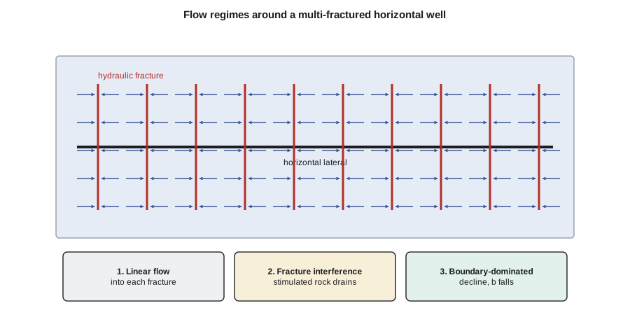
Production follows a characteristic sequence. In the first days to weeks the fracture network itself drains, together with load water from the treatment. Then comes a long period of linear flow from the matrix into the fracture faces, during which the rate declines roughly as one over the square root of time. When the pressure disturbances from adjacent fractures meet, the rock between them begins to deplete as a unit and the decline steepens toward boundary-dominated flow. For the Caribou Ridge wells, rate-transient analysis of the four existing wells shows linear flow lasting about two to three years.

Decline curves: Arps and its limits

Arps' 1945 decline equations remain the industry's basic forecasting tool. The hyperbolic form is:

with the initial rate q_i, the initial nominal decline D_i and the exponent b. For b = 0 the equation becomes exponential decline, and for b = 1 harmonic decline. Arps derived the forms for boundary-dominated flow, where b lies between 0 and 1. Tight and shale wells in linear flow fit b values of 1.5 to 2 or more, and applying such a b-factor for the whole life of a well predicts a cumulative production that grows without limit. Reserves evaluators therefore use a modified hyperbolic decline: hyperbolic with a high b until the decline rate falls to a terminal value, typically 5 to 10 percent per year, and exponential after that. Other models, such as the stretched exponential (Valkó) and Duong's model built for linear flow, are used alongside Arps, and evaluators under COGEH and NI 51-101 must justify the parameters with analogue wells.

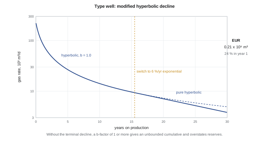
Ethan's type well uses an initial rate of 227 × 10³ m³/d (8.0 MMscf/d), an initial decline of 150 percent per year (nominal), b = 1.0 and a terminal decline of 6 percent per year. The model switches to exponential decline after about 15 years. The first year produces about 50 million m³ (1.8 Bscf), and the 30-year estimated ultimate recovery, EUR, is about 208 million m³ (7.4 Bscf) of raw gas, with about a quarter in year one. That front-loading is typical of shale and tight wells, and it is why their economics depend so strongly on the first year's rate and on drilling a steady stream of new wells to keep a plant full.

Spacing, parent-child effects and recovery

The most consequential decision in a tight gas development is how many wells to place in each spacing unit. More wells recover more of the gas in place, but each additional well recovers less, because its drainage area overlaps its neighbours'. Wells drilled next to older, partly depleted wells, the parent-child problem, often underperform, because the new fractures grow toward the depleted rock. Ethan's code shows that four wells per 259-ha spacing unit in one landing zone would recover about 48 percent of the free gas in place in that zone. The team will test closer and wider spacing with two pilot pads and with microseismic and pressure monitoring before committing to a full-field pattern.

Gas engineers also watch the water. Each Caribou Ridge well uses tens of thousands of cubic metres of water for fracturing. In British Columbia, water licensing, recycling of flowback and produced water, and disposal by deep injection are all regulated by the BCER, and most operators now recycle a large share of their flowback. Induced seismicity from fracturing and disposal has led to traffic-light protocols in some areas, under which operations must slow or stop if events above set magnitudes occur. These are part of the development plan as much as the decline curve is.