Waterflood design

Every EOR project in a light oil pool inherits a waterflood: its wells, its patterns, its injection water and its history. Before Ethan can design a tertiary process, he needs to understand the waterflood design decisions made when the Cardium A waterflood pilot was expanded, and whether they still make sense. Lena suggests he rebuild the design calculations from scratch, “the way we would have done them in 1970,” and then compare them with the simulation. The classical methods are fast, transparent and still used to check simulation results and to screen new floods.

Why waterflood

Water is the cheapest and most widely available injectant. It is denser than oil, so it tends to sweep the lower part of a formation, and in most light oil reservoirs its mobility ratio is favourable. Waterflooding has been the dominant secondary recovery method since the 1950s, and today most of the world's light oil production comes from fields under waterflood or natural water drive. Good waterflood candidates have a reasonably continuous reservoir, an oil viscosity low enough for a favourable or moderate mobility ratio, a remaining oil saturation well above residual, and a nearby water source. Floods that start while the pressure is still above or near the bubble point avoid the large free gas saturations that delay response.

Flood patterns

Wells are arranged in repeating patterns of injectors and producers. In a direct line drive, rows of injectors face rows of producers; in a staggered line drive, the rows are offset by half a spacing. In a five-spot, each injector sits at the centre of a square of four producers and each producer at the centre of four injectors, so there is one injector per producer. A seven-spot has two producers per injector and a nine-spot three. The inverted nine-spot, with one injector at the centre of eight producers, is popular in early development because it begins with many producers and few injectors and can later be converted to a five-spot or line drive by turning producers into injectors. Peripheral and crestal floods inject along the edges or the top of a structure and are suited to dipping reservoirs with good continuity.

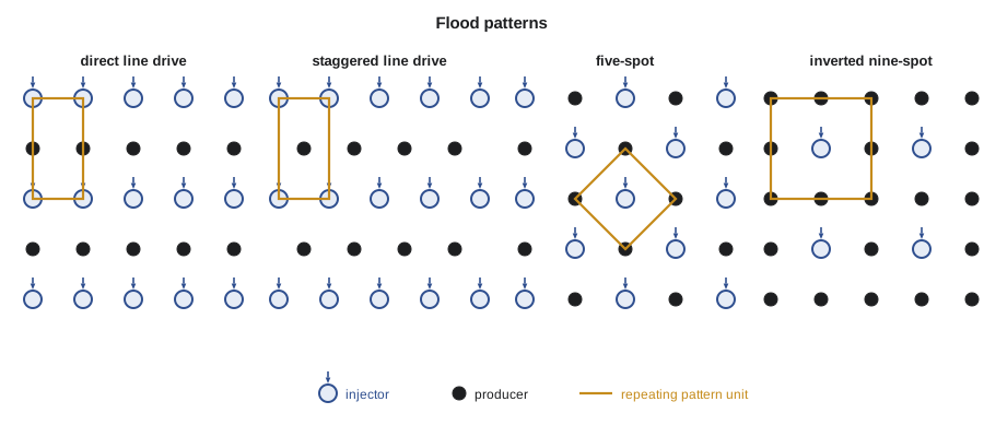
The choice of pattern balances several factors. The ratio of producing to injecting wells should match the ratio of the fluids' injectivity and productivity: if injectors take water poorly, more injectors per producer are needed. Pattern alignment matters in reservoirs with directional permeability or natural fractures; injectors and producers should not be aligned along the high-permeability direction, or water will channel straight across. The existing wells usually dominate the decision, because converting a producer is far cheaper than drilling an injector. Modern floods in tight rock often use horizontal wells, either as long horizontal injectors and producers in alternating parallel lines or as horizontal producers paired with vertical injectors.

Injectivity

Injection rate is limited by the injection pressure, which must stay below the formation parting pressure unless fractured injection is planned, and by the pattern's ability to take water. For a five-spot with unit mobility ratio, Muskat's analytical solution gives the injection rate per injector:

in consistent units, where d is the distance from injector to producer and Δp the pressure difference between their bottomholes. Deppe and later authors extended the result to other patterns and mobility ratios. Injectivity in a real flood changes with time. It falls during the fill-up period as the oil bank forms, and in a favourable flood it then falls further because the water must push a growing bank of less mobile oil; in an unfavourable flood it rises after breakthrough. Water quality affects it too: suspended solids, oil droplets and bacteria plug the sandface, so injection water is filtered, deaerated and treated.

Many waterfloods inject above the parting pressure deliberately, especially in low-permeability rock, so that each injector develops a short induced fracture that greatly improves injectivity. The fractures must be kept short and oriented sensibly with respect to the producers; uncontrolled fracture growth toward a producer is one of the main causes of poor waterflood sweep. A step-rate test, injecting at increasing rates and watching for a break in the pressure-rate plot, finds the parting pressure for each injector.

Buckley-Leverett and Welge, briefly

PET-320 developed the Buckley-Leverett theory of one-dimensional displacement. The water fractional flow, neglecting gravity and capillary pressure, is f_w = 1 / (1 + (k_ro μ_w) / (k_rw μ_o)). Each saturation travels at a speed proportional to the slope of the fractional flow curve, and because slow, low saturations would be overtaken by faster, higher ones, a shock forms at the front. Welge's construction finds the shock: a tangent to the f_w curve drawn from the initial water saturation touches it at the front saturation S_wf, and extends to f_w = 1 at the average saturation behind the front. At breakthrough the pore volumes injected are the reciprocal of the tangent's slope.

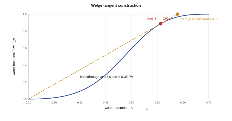
After breakthrough, the outlet saturation S_w2 rises above S_wf. The pore volumes injected are Q_i = 1 / f_w′(S_w2), and the average saturation is:

so the displacement efficiency is (S̄_w − S_wc) / (1 − S_wc). This gives oil recovery from a single linear layer as a function of throughput, which is the building block of all the classical forecasting methods.

# Waterflood design: Buckley-Leverett/Welge performance and five-spot injectivity.
import math
SI = True      # True: metric units, False: oilfield units

swc, sor, kro0, krw0, no, nw = 0.30, 0.28, 0.80, 0.30, 2.5, 2.0
mu_o, mu_w = (0.72 if SI else 0.95), 0.50

def fw(sw):
    s = min(max((sw - swc) / (1 - swc - sor), 0.0), 1.0)
    lw, lo = krw0 * s ** nw / mu_w, kro0 * (1 - s) ** no / mu_o
    return lw / (lw + lo) if lw + lo > 0 else 1.0

def dfw(sw, h=1e-5): return (fw(sw + h) - fw(sw - h)) / (2 * h)

# Welge tangent from (swc, 0): maximize fw / (sw - swc)
grid = [swc + 1e-4 + i * (1 - sor - swc) / 4000 for i in range(4001)]
swf = max(grid[1:-1], key=lambda s: fw(s) / (s - swc))
sbar = swc + 1 / dfw(swf)
print(f"Front saturation {swf:.3f}, fw at front {fw(swf):.3f}")
print(f"Breakthrough at {1 / dfw(swf):.3f} PV, average Sw {sbar:.3f}, E_D {(sbar - swc) / (1 - swc):.3f}")
# after breakthrough: pick sw2 > swf, Qi = 1 / f'(sw2), sbar = sw2 + (1 - fw) Qi
for target in (0.5, 1.0, 2.0, 3.0):
    sw2 = min((s for s in grid if swf < s < 1 - sor - 0.003), key=lambda s: abs(1 / dfw(s) - target))
    qi = 1 / dfw(sw2); sb = sw2 + (1 - fw(sw2)) * qi
    print(f"  {qi:4.2f} PV injected: water cut {fw(sw2):.3f}, E_D {(sb - swc) / (1 - swc):.3f}")

# Five-spot injectivity at unit mobility ratio (Muskat): q = pi k h dp / (mu (ln(d/rw) - 0.619))
k = 15e-15; h = 6.5; dp = 8.0e6; rw = 0.089
area = 16.2e4                       # pattern area, m2 (40 acres)
d = math.sqrt(area / 2)             # injector-producer distance
q = math.pi * k * h * dp / (mu_w * 1e-3 * (math.log(d / rw) - 0.619)) * 86400
if SI:
    print(f"Pattern 16.2 ha, d = {d:.0f} m, injection rate about {q:.0f} m³/d at a pressure difference of 8,000 kPa")
else:
    print(f"Pattern 40 acres, d = {d / 0.3048:.0f} ft, injection rate about {q * 6.2898:.0f} bbl/d at a pressure difference of 1,160 psi")

Front saturation 0.608, fw at front 0.887
Breakthrough at 0.347 PV, average Sw 0.647, E_D 0.495
  0.50 PV injected: water cut 0.936, E_D 0.514
  1.00 PV injected: water cut 0.977, E_D 0.541
  2.00 PV injected: water cut 0.992, E_D 0.560
  3.00 PV injected: water cut 0.996, E_D 0.569
Pattern 16.2 ha, d = 285 m, injection rate about 57 m³/d at a pressure difference of 8,000 kPa

The output shows a typical light oil waterflood. Breakthrough comes at about a third of a pore volume, with half the oil in the swept rock already displaced, and afterwards the water cut climbs rapidly while the displacement efficiency inches upward. By three pore volumes the water cut is above 99 percent, and the remaining improvement is too slow to pay for the water handling. The injectivity estimate, about 57 m³/d per injector at a moderate pressure difference, is in line with the rates the Cardium A waterflood pilot achieved.

From one layer to a pattern

Buckley-Leverett treats one linear layer. A pattern forecast must add areal sweep and layering. Two classical methods do this. The Stiles method of 1949 treats the reservoir as layers of different permeability, each with piston-like displacement and the same mobility, and orders them by breakthrough time; it is essentially the Dykstra-Parsons approach with M = 1, applied to produce a water-oil ratio and recovery as functions of time. The Craig-Geffen-Morse method of 1955 combines Buckley-Leverett frontal advance with the scaled-model areal sweep data for a five-spot, including the growth of areal sweep after breakthrough. It accounts for the period before fill-up when an initial gas saturation is present, and it predicts oil rate, water rate and injectivity through the life of a pattern.

Craig's 1971 SPE monograph, The Reservoir Engineering Aspects of Waterflooding, compares these and other methods against field results and is still the standard reference. Its conclusion holds today: methods that combine fractional flow, areal sweep and layering predict field performance reasonably well; methods that ignore any one of the three can be badly wrong. Modern practice uses numerical simulation for the final design, but streamline models and the classical methods remain valuable for quick screening and for checking that a simulation result is physically plausible.

Water source and treatment

A waterflood needs a reliable water supply for decades, typically one to two reservoir barrels of water injected for every reservoir barrel of fluid produced over the life of the flood, including make-up for the voidage of produced oil and gas. Produced water is reinjected wherever possible, and the make-up water comes from a source formation, surface water or, increasingly, saline aquifers that do not compete with fresh water uses. Mixing incompatible waters can precipitate scale, so a compatibility study checks for barium and strontium sulphate and calcium carbonate precipitation. Oxygen is removed to limit corrosion, and biocides control sulphate-reducing bacteria, which can sour a reservoir with hydrogen sulphide. These details matter for EOR as well: polymer and surfactant performance depend strongly on water salinity and hardness.

Ethan's rebuild of the classical design agrees with the simulation within ten percent for the pilot pattern's recovery at a water cut of 95 percent, which gives him confidence in both. More importantly, it shows him which assumption controls the answer: the layering. The next step is to see how the field has actually behaved, which is the subject of Lesson 5.

One practical rule closes the design discussion. Before a pattern flood is committed across a pool, most operators convert a single injector or a small group and watch the offset producers for six to twelve months. The response time, the change in producing gas-oil ratio and the first water arrivals calibrate the design calculations far better than any amount of laboratory data, and they reveal directional permeability and barriers early.