
PET-430 · Lesson 12 of 12 · 19 min
EOR economics and capstone
A year after Lena's question, Ethan presents his recommendation to the Prairie Crest management committee in Calgary. He has screened the Cardium A pool, worked through the laboratory results with Mei Lin, rebuilt the waterflood design, diagnosed the thief layer with the field team at Drayton Valley, and run the history-matched model for every process that passed the screen. This capstone lesson follows the last step: turning the technical work into an economic comparison and a staged plan that a company can act on. It draws on every earlier lesson, and it shows that the best EOR process is not always the one that recovers the most oil.
What makes EOR economics different
EOR projects share several features that set their economics apart from drilling new wells. First, they are incremental: the value of the project is the difference between the forecast with EOR and the forecast without it, so the waterflood base case must be forecast just as carefully as the EOR case, and both come from the same model. Second, they are front-loaded: injection facilities, recycle plants, pipelines and well conversions are paid for before the oil response arrives, typically one to three years later. Third, they carry a large and continuing injectant cost, whether CO2, polymer or surfactant, which behaves like an operating cost per barrel and makes the project sensitive to oil price. Fourth, they are long: a CO2 or chemical flood runs for 15 to 30 years, so the discount rate strongly affects the answer.
The usual measures are those of PET-450: net present value at the company's discount rate, internal rate of return, payout time and capital efficiency, expressed as NPV per unit of capital invested. For EOR two further measures are common. The injectant cost per incremental barrel, the net utilization of Lesson 7 multiplied by the injectant price, is the quickest way to compare processes and fields. The breakeven oil price is the price at which the NPV is zero; projects with a breakeven well below the company's planning price are robust.
Screening the pool: a summary
| Process | Screen | Main technical issue in the pool | Status |
|---|---|---|---|
| CO2 miscible WAG | passes | Pressure at MMP; thief layer; CO2 supply | Candidate |
| Hydrocarbon miscible gas | passes | Gas supply limited; enrichment needed | Not pursued |
| Polymer flooding | passes | Favourable M already; helps thief layer | Candidate, as conformance |
| Surfactant-polymer | passes | Retention in clay-bearing sand; salinity control | Candidate, high risk |
| Low-salinity water | uncertain | Clays present; source water needed | Laboratory test |
| Nitrogen | fails | MMP far above reservoir pressure | Rejected |
| Thermal methods | fails | Light oil, depth, permeability | Rejected |
Three options reach the economic comparison. The first is a CO2 WAG flood, with average pressure raised about ten percent above the slim-tube MMP of Lesson 6, a tapered WAG ratio near 1:1 and 0.6 HCPV of CO2, forecast to recover about 12 percent of the original oil in place. The second is a polymer conformance flood aimed at the thief layer, using a deep-placed gel at the worst injectors and then polymer at about 10 mPa·s (10 cp), forecast to recover about 3 percent. The third is a surfactant-polymer flood, forecast to recover about 10 percent but with the retention and salinity risks of Lesson 10.
# Capstone economics: three EOR options for the pool, with NPV, payback and a pilot decision.
import math
SI = True      # True: Canadian case (metric reporting), False: US case (oilfield reporting)
BBL = 6.2898
ooip_bbl = 5.68e6 * BBL                         # original oil in place, bbl
price = 90.0 if SI else 70.0                    # dollars per bbl
roy = 0.15 if SI else 0.25                      # royalty and production taxes
co2_cost = 40.0                                 # dollars per tonne delivered
credit = 0.0 if SI else 30.0                    # storage credit passed to the operator, dollars per tonne
rate = 0.10

opts = {   # name: (fraction of OOIP, delay yr, tau yr, capex M, opex dollars/bbl, injectant dollars/bbl)
    'CO2 WAG':              (0.120, 1, 4.0, 80.0, 14.0, 0.32 * (co2_cost - credit)),
    'polymer conformance':  (0.030, 1, 3.0, 15.0, 10.0, 4.0),
    'surfactant-polymer':   (0.100, 2, 4.0, 70.0, 14.0, 22.0),
}
def profile(frac, delay, tau, years=20):
    sh = [max(t - delay, 0) * math.exp(-max(t - delay, 0) / tau) for t in range(1, years + 1)]
    return [ooip_bbl * frac * s / sum(sh) for s in sh]

res = {}
for name, (frac, d, tau, capex, opex, inj) in opts.items():
    oil = profile(frac, d, tau)
    cf = [-capex * 0.6e6, -capex * 0.4e6] + [0.0] * 18
    for t, q in enumerate(oil):
        cf[t] += q * (price * (1 - roy) - opex - inj)
    npv = sum(c / (1 + rate) ** (t + 0.5) for t, c in enumerate(cf))
    cum, pay = 0.0, None
    for t, c in enumerate(cf):
        cum += c
        if pay is None and cum > 0: pay = t + 1
    res[name] = npv
    vol = f"{sum(oil) / BBL / 1e6:.2f} million m³" if SI else f"{sum(oil) / 1e6:.2f} MMbbl"
    print(f"{name:20s} oil {vol:16s} NPV10 {npv / 1e6:6.1f} M, NPV/capex {npv / (capex * 1e6):4.2f}, payout year {pay}")

# Pilot first? CO2: pilot 8 M, success probability 0.6; failure after a full project loses 70 % of capex
p, pilot = 0.6, 8.0e6
go_now = p * res['CO2 WAG'] + (1 - p) * (-0.7 * opts['CO2 WAG'][3] * 1e6)
with_pilot = -pilot + p * res['CO2 WAG'] / 1.1 ** 2
print(f"CO2 full project now, expected value {go_now / 1e6:5.1f} M; pilot first {with_pilot / 1e6:5.1f} M")
print("Currency: " + ("Canadian dollars" if SI else "US dollars"))CO2 WAG oil 0.68 million m³ NPV10 36.4 M, NPV/capex 0.46, payout year 6 polymer conformance oil 0.17 million m³ NPV10 25.0 M, NPV/capex 1.66, payout year 4 surfactant-polymer oil 0.57 million m³ NPV10 4.1 M, NPV/capex 0.06, payout year 8 CO2 full project now, expected value -0.5 M; pilot first 10.1 M Currency: Canadian dollars
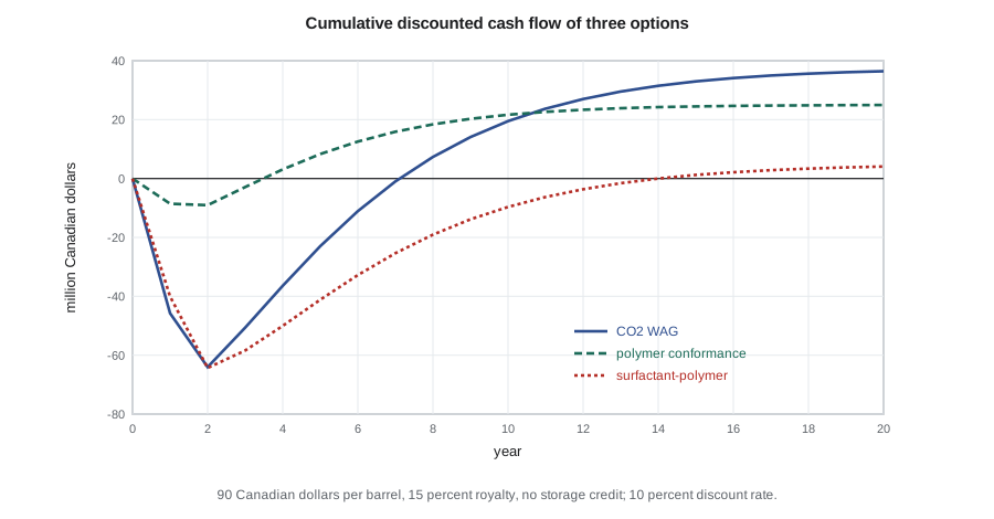
The results frame the decision. The CO2 flood has the largest NPV, about 36 million Canadian dollars, but it also needs the most capital and pays out only in its sixth year. The polymer conformance project is much smaller but has by far the best capital efficiency, with an NPV of about 1.7 times its capital and payout in year four. The surfactant-polymer flood barely breaks even once its chemical costs are counted, and that is before its technical risk is considered. The expected-value calculation adds a further point: with a 60 percent chance of technical success, committing to the full CO2 project now has an expected value near zero, while a pilot first, at 8 million dollars, raises the expected value to about 10 million by avoiding a large loss if the pilot fails.
Worked problem
Injectant cost per incremental barrel
The CO2 flood has a net utilization of 0.32 tonnes of purchased CO2 per incremental barrel. Delivered CO2 costs 40 dollars per tonne. No storage credit is assumed in the Canadian case. (In the US case, 30 dollars per tonne of the storage credit is assumed to be passed to the operator.) Find the injectant cost per incremental barrel and the netback after royalties, operating cost of 14 dollars per barrel and injectant, at 90 dollars per barrel with 15 percent royalty (70 dollars per barrel with 25 percent royalty and taxes).
Show solution
- Net CO2 cost per tonne is 40 − 0 = 40 (40 − 30 = 10) dollars.
- Injectant cost per barrel is 0.32 × 40 = 12.80 (0.32 × 10 = 3.20) dollars.
- Revenue after royalty is 90 × 0.85 = 76.50 (70 × 0.75 = 52.50) dollars per barrel.
- The netback is 76.50 − 14.00 − 12.80 = 49.70 (52.50 − 14.00 − 3.20 = 35.30) dollars per incremental barrel.
Answer: The netback is about 50 (35) dollars per incremental barrel before capital. The injectant is the second largest cost after royalties, so a cheaper CO2 source or a storage credit would change the economics substantially. (Even with the credit, the lower price and higher royalty burden leave a thinner margin than the operating and injectant costs alone suggest.)
Risk and the value of a pilot
Every EOR forecast carries large uncertainty: the sweep in the thief layer, the response time, the injectant utilization, and the oil price over 20 years. The PET-420 forecast for the waterflood pilot already had a P10 roughly twice its P90, and an EOR forecast built on top of it is wider still. A field pilot is a way of buying information. It costs money and time, but it can reveal a fatal flaw, such as early CO2 breakthrough through the thief layer or unacceptable surfactant retention, before the full investment is made. Pilots must be designed to answer specific questions: an inverted five-spot or a pair of patterns with observation wells, tracers and logging, and a clear definition in advance of what result would justify expansion.
Phasing is the other risk tool. A project can be developed pattern by pattern, starting where the reservoir is best understood and the surface facilities closest, so that early patterns' performance guides later ones and early cash flow helps fund expansion. Phasing reduces peak capital exposure and makes good use of recycle capacity, at the cost of some delay in the full benefit.
Ethan's recommendation
Ethan's recommendation has three stages. First, start the polymer conformance programme now: gel treatments at the three injectors connected to the thief layer, followed by polymer injection in the affected patterns. It is cheap, pays out quickly, and improves the sweep that any later process will rely on. Second, raise the average pool pressure above the MMP by running the waterflood at a voidage replacement ratio near 1.1, and negotiate for captured CO2 from the Alberta Carbon Trunk Line system or another nearby source. Third, run a two-pattern CO2 WAG pilot with an observation well and tracers in the best-characterized part of the pool, with expansion conditional on CO2 breakthrough later than 0.3 HCPV and net utilization below 2.5 tonnes per cubic metre. Surfactant-polymer flooding stays in the laboratory until retention can be cut, and low-salinity water is tested in cores alongside it.
Lena's comment after the meeting is the last word of the course. “You did not recommend the process with the biggest number. You recommended the one we can afford to be wrong about, and you set up the test that tells us whether the big one is real. That is what EOR engineering is.” The committee approves the conformance programme and funds the CO2 supply study.
Sensitivities and the breakeven price
Before the meeting, Lena asks Ethan to test how robust each option is. He reruns the economics with oil price 20 percent lower, injectant costs 20 percent higher, incremental recovery 30 percent lower and a one-year delay in response, one at a time. The incremental recovery has the largest effect for every option, followed by oil price. The CO2 flood is the most sensitive to price because its injectant cost is fixed per tonne while revenue falls; the polymer conformance project is the least sensitive because its capital is small and its response is quick. The surfactant-polymer flood loses most of its value under any single adverse change.
He also computes the breakeven oil price of each option by searching for the price at which the NPV is zero. A short loop over prices in steps of one dollar is enough, and the result is easy to communicate: a project whose breakeven price is well below the company's long-term planning price can survive a downturn, while one whose breakeven is close to it is a bet on price. Ethan's chart of breakeven prices becomes the single slide the committee discusses longest.
Two further points come up in discussion. The first is timing: the value of an EOR project depends on starting it while the waterflood infrastructure, wells and pipelines are still in good condition and before the pool's production falls to its economic limit. Waiting has a cost, because the base case declines and wells are abandoned, and a project that is marginal today may be impossible in ten years. The second is portfolio fit: a large CO2 project would take most of the company's capital for two years, while the conformance programme leaves room for drilling elsewhere. Both points favour the staged plan.
Common mistakes
MistakeValuing an EOR project on total rather than incremental oil.
InsteadSubtract the waterflood base case; only the incremental oil and costs belong to the project.
MistakeChoosing the option with the largest recovery.
InsteadCompare NPV, capital efficiency, payout and risk; the biggest resource is often not the best first project.
MistakeRunning a pilot without success criteria.
InsteadDefine in advance which measured results justify expansion, and design the pilot to measure them.
MistakeIgnoring the injectant cost per barrel.
InsteadNet utilization times injectant price is often the largest controllable cost and the best comparison between processes.
Summary and key terms
- EOR value is incremental over a carefully forecast waterflood base case.
- EOR projects are front-loaded, long and sensitive to oil price and injectant cost.
- NPV, capital efficiency, payout, injectant cost per barrel and breakeven price are the key measures.
- Pilots buy information that can prevent large losses; they need clear objectives and success criteria.
- Phased development reduces capital exposure and uses early results to guide expansion.
- For the pool, a staged plan starts with cheap conformance work and tests the larger CO2 option before committing.
- Incremental oil
- Oil produced with the EOR project minus oil the base case would have produced.
- Capital efficiency
- NPV per unit of capital invested.
- Breakeven price
- The oil price at which the project NPV is zero.
- Netback
- Revenue per barrel after royalties, operating costs and injectant costs.
- Value of information
- The increase in expected value from obtaining information, such as a pilot result, before deciding.
- Phased development
- Expanding a project in stages, using results from early stages to guide later ones.
- Success criteria
- Measured results, set in advance, that justify expanding a pilot.
Practice problems
Work each problem on paper first, then reveal the answer to check.
Why must the base case be forecast as carefully as the EOR case?
Show answer
The project's value is the difference between them, so an error in either is an error in the value.
Net utilization is 0.25 t/bbl and CO2 costs 50 dollars per tonne. What is the CO2 cost per barrel?
Show answer
0.25 × 50 = 12.50 dollars per barrel.
A project has NPV of 20 million on capital of 80 million. What is its capital efficiency?
Show answer
20 / 80 = 0.25.
Name two questions a CO2 pilot in the pool should answer.
Show answer
When CO2 breaks through, given the thief layer, and what the net utilization is; incremental oil response and injectivity are others.
Lesson quiz · 5 questions
Score 60% or more to complete this lesson.
Create a free account to save your progress, take quizzes and earn a certificate.