Mechanistic models

Ethan's comparison in lesson 7 left one result unexplained. The mechanistic model matched the north pad line better than any correlation, but he had used it as a black box. Mei Lin, the flow assurance specialist who supports Prairie Crest from the Calgary office, offers to walk him through how such a model works. 'A mechanistic model is just a collection of simple physical balances, one for each flow pattern,' she says. 'Once you see the pieces, you will know when to trust it and when not to.'

This lesson explains the structure of mechanistic models for steady multiphase flow: a flow pattern prediction from physical transition criteria, followed by a separate momentum balance for each pattern. It develops the two-fluid model for stratified flow and the slug unit model for slug flow, introduces the unified models used in current software, and briefly describes transient simulators.

The structure of a mechanistic model

Empirical correlations fit holdup and friction directly to data. Mechanistic models instead start from the physics of each flow pattern. They first predict the pattern from transition criteria like those of Taitel and Dukler (lesson 4) and Taitel, Barnea and Dukler (lesson 5). Then, for the predicted pattern, they solve a simplified momentum balance on each phase, or on the slug unit, with closure relations for wall and interfacial shear, slug velocities, bubble rise and droplet entrainment. The closure relations are themselves partly empirical, but they describe local physics such as the shear on a film or the rise of a bubble, which can be measured in the laboratory and is expected to scale to field conditions better than a whole-line correlation.

The best-known comprehensive models include those of Ansari and coworkers (1994) for vertical wells, Xiao, Shoham and Brill (1990) for pipelines, Petalas and Aziz (2000), which drew on the large Stanford multiphase flow database, and the Tulsa University Fluid Flow Projects unified model of Zhang and coworkers (2003). Commercial steady-state simulators use these or proprietary methods, often called point models, at each segment of a pipe.

The two-fluid model for stratified flow

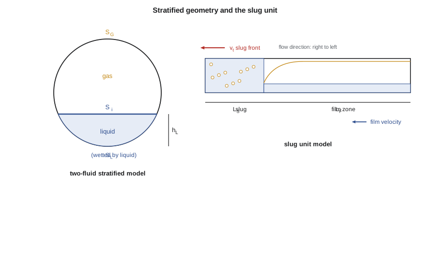
In stratified flow, the liquid and gas occupy separate parts of the pipe cross-section, divided by an interface at height h_L. A momentum balance on each phase, for steady fully developed flow, gives:

Here A_L and A_G are the areas occupied by each phase, S_L, S_G and S_i the wetted perimeters of liquid, gas and interface, τ_WL and τ_WG the wall shear stresses, and τ_i the interfacial shear stress. All the areas and perimeters are functions of h_L / D through the geometry of a circle. The wall stresses are calculated from single-phase friction factors using hydraulic diameters for each phase; the interfacial stress uses a friction factor that is equal to the gas wall value for a smooth interface and larger for a wavy one.

Eliminating the pressure gradient between the two equations leaves a single equation in the liquid level h_L / D. Solving it gives the level, and from the level the holdup, the actual velocity of each phase and finally the pressure gradient. Taitel and Dukler showed that, for given dimensionless groups, the equation has a unique solution for most practical conditions, which makes it convenient for computation.

# Two-fluid model of stratified flow: find the liquid level that balances the shear stresses (Taitel-Dukler style)
import math
SI = True   
g = 9.81
D = 0.154; A = math.pi * D * D / 4
rhoL, rhoG, muL, muG = 880.0, 15.0, 0.003, 1.2e-5
vsl, vsg = 0.05, 1.5
theta = math.radians(0.5)             # slight downhill angle of a line falling toward a creek crossing (positive = downward)
def geom(hD):
    a = 2 * math.acos(1 - 2 * hD)                 # wetted angle
    AL = A * (a - math.sin(a)) / (2 * math.pi); AG = A - AL
    SL = D * a / 2; SG = D * math.pi - SL; Si = D * math.sin(a / 2)
    return AL, AG, SL, SG, Si
def fr(Re, laminar, turb):
    return (16 / Re) if Re < 2000 else turb[0] * Re ** -turb[1]
def residual(hD):
    AL, AG, SL, SG, Si = geom(hD)
    vL, vG = vsl * A / AL, vsg * A / AG
    DL = 4 * AL / SL; DG = 4 * AG / (SG + Si)
    fL = fr(rhoL * vL * DL / muL, 1, (0.046, 0.2)); fG = fr(rhoG * vG * DG / muG, 1, (0.046, 0.2))
    tL = fL * rhoL * vL * vL / 2; tG = fG * rhoG * vG * vG / 2; ti = fG * rhoG * (vG - vL) * abs(vG - vL) / 2
    return tG * SG / AG - tL * SL / AL + ti * Si * (1 / AL + 1 / AG) + (rhoL - rhoG) * g * math.sin(theta)
lo, hi = 0.01, 0.99
for _ in range(80):
    mid = (lo + hi) / 2
    if residual(lo) * residual(mid) <= 0: hi = mid
    else: lo = mid
hD = (lo + hi) / 2
AL, AG, *_ = geom(hD)
HL = AL / A
print(f"equilibrium liquid level h/D = {hD:.3f}, liquid holdup {HL:.3f} (no-slip value {vsl / (vsl + vsg):.3f})")
f = 1 if SI else 3.2808; u = "m/s" if SI else "ft/s"
print(f"actual liquid velocity {vsl / HL * f:4.2f} {u}, actual gas velocity {vsg / (1 - HL) * f:4.2f} {u}")
# Slug unit: translational velocity and a simple liquid balance
vm = 2.0; C0, vd = 1.2, 0.54 * math.sqrt(g * D)
vt = C0 * vm + vd
HLs, HLf = 0.85, 0.15
print(f"slug front velocity for vm {vm * f:.1f} {u}: {vt * f:4.2f} {u}")
beta = (HLs - 0.35) / (HLs - HLf)          # fraction of the unit that is film, for an average holdup of 0.35
print(f"with slug holdup {HLs}, film holdup {HLf} and average 0.35, the film occupies {beta:.0%} of each slug unit")

equilibrium liquid level h/D = 0.143, liquid holdup 0.088 (no-slip value 0.032)
actual liquid velocity 0.57 m/s, actual gas velocity 1.64 m/s
slug front velocity for vm 2.0 m/s: 3.06 m/s
with slug holdup 0.85, film holdup 0.15 and average 0.35, the film occupies 71% of each slug unit

For the late-life north pad conditions, Ethan's code finds a liquid level of only 14 percent of the diameter, a holdup of 0.088 against a no-slip value of 0.032, and a liquid velocity of 0.57 m/s against 1.64 m/s for the gas. 'So the liquid is moving at about a third of the gas speed,' Mei says. 'That is slip, calculated from shear and gravity rather than fitted. And notice the line is slightly downhill here. On the next uphill the level will rise sharply.'

The slug unit model

Slug flow is modelled by treating it as a repeating unit: a liquid slug of length L_S, which may contain small gas bubbles, followed by a film zone of length L_F, where a long gas bubble rides over a liquid film. The total unit length is L_U = L_S + L_F. The slug front moves at a translational velocity that is faster than the mixture velocity because the slug picks up the slow film ahead of it:

Here C₀ is about 1.2 for turbulent flow, reflecting the faster liquid near the pipe centre, and v_d is a drift velocity, which in horizontal pipes is small and in inclined pipes is related to 0.35√(gD) and 0.54√(gD) through the inclination. A mass balance on the liquid over the unit, together with the holdup in the slug body H_LS and in the film H_LF, gives the fraction of each unit occupied by the film. The pressure gradient is then the weighted sum of friction and gravity in the slug body and the film zone.

The slug body holdup is one of the most important closure relations. Gregory, Nicholson and Aziz, in 1978, correlated it against mixture velocity, giving values near 1 at low velocity and falling to about 0.5 at high velocity as the slug becomes aerated. Slug length is another: observations in horizontal pipes suggest stable slugs are about 30 pipe diameters long for small pipes, but field data in large-diameter lines show much longer slugs, and the distribution of lengths matters for separator design. Lesson 11 returns to slug lengths and slug catchers.

In Ethan's example, a mixture velocity of 2.0 m/s gives a translational velocity of about 3.1 m/s. With a slug holdup of 0.85, a film holdup of 0.15 and an average holdup of 0.35, the film occupies about 71 percent of each unit. Most of the line, at any moment, is film zone, while most of the liquid travels in the slugs.

Bubble, annular and dispersed bubble models

For bubble and dispersed bubble flow, mechanistic models use a drift-flux form (lesson 5), with a bubble rise velocity and a distribution parameter. For annular flow, they solve momentum balances for the liquid film and the gas core, with closure relations for the interfacial shear, which increases strongly with film thickness because the film surface is rough with waves, and for the fraction of liquid entrained as droplets. Entrainment correlations, such as those of Ishii and Mishima and of Oliemans and coworkers, are among the least certain parts of annular flow models, but they matter most in gas-condensate lines, where much of the liquid can travel as droplets.

Unified models

The original mechanistic models treated each pattern with its own equations and switched between them at the predicted transitions, which can cause discontinuities: the predicted pressure gradient may jump when the pattern changes. Unified models, such as the Tulsa model of Zhang and coworkers, address this by treating slug flow as the central pattern and deriving the transitions from the slug unit itself. Stratified or annular flow appears as the limit where the slug length goes to zero, and dispersed bubble flow as the limit where the film zone disappears. The result is a continuous model that is easier to use in optimization and network calculations.

Transient models

Steady-state models describe average behaviour. They cannot predict how a line responds to a shut-in and restart, to pigging, to rate changes or to severe slugging cycles. Transient multiphase simulators, such as OLGA, LedaFlow and others, solve time-dependent conservation equations for mass, momentum and energy of each phase or field (gas, liquid film and droplets) along the pipe, with closure relations similar to those of steady mechanistic models. They are used for flow assurance studies: pig slug arrival volumes, terrain slugging, cooldown times after shutdown, and hydrate and wax risk during transient operations. Lesson 11 uses results of the kind such tools produce, though the calculations there are simplified.

Strengths and limits

Mechanistic models generally extrapolate better than empirical correlations to pipe sizes, pressures and fluids outside the range of the laboratory data, because their closure relations describe local physics. Comparisons against large databanks have often found them to give lower average errors, especially for inclined flow and gas-condensate systems. They are not perfect. Their closure relations were also developed largely in small pipes with air and water, the transition criteria carry uncertainty, and slug length and entrainment remain hard to predict. A mechanistic model should be checked against field data just as a correlation is, as Ethan did in lesson 7.

A worked check by hand

Even when the software does the work, an engineer can check a mechanistic result with a few hand calculations. For stratified flow, check that the predicted liquid velocity is less than the gas velocity and that the liquid level is reasonable for the inclination; on a downhill segment, a low level and fast liquid are expected. For slug flow, check that the translational velocity is about 1.2 times the mixture velocity, that the slug body holdup is between 0.5 and 1, and that the average holdup lies between the film and slug values. For annular flow, check that the gas velocity is above the critical value of lesson 5. Results that fail these checks suggest an input error, such as a wrong unit or inclination, more often than a model failure.