
PET-380 · Lesson 6 of 12 · 19 min
The homogeneous model and pressure gradient components
Marisol has one more request before Ethan returns to the gathering line. 'Before you use the big correlations,' she says, 'build the simplest possible model yourself, so you know what the correlations are adding.' She hands him the 03-22 completion: 62 mm (2.441 in) tubing to about 2,400 m vertical depth, 90 m³/d of oil, 45 m³/d of water and a producing gas-oil ratio of 150 m³/m³. 'Assume the gas and liquid move together with no slip. Then tell me how much of the pressure drop is gravity, how much is friction and how much is acceleration.'
This lesson develops the general pressure gradient equation for multiphase flow, separates it into its gravity, friction and acceleration components, and applies the homogeneous no-slip model, which treats the mixture as a single pseudo-fluid. It then shows how to march the calculation along a pipe in steps, because fluid properties change with pressure and temperature.
The general pressure gradient equation
A momentum balance on a short length of pipe of length dL, inclined at angle θ from horizontal, gives the steady-state pressure gradient as the sum of three parts:
The first term is the gravity or elevation gradient: the weight of the fluid column per unit length, using the in-situ (slip) density ρ_s = ρ_L H_L + ρ_G (1 − H_L). The second is the friction gradient, written in the Darcy-Weisbach form with a friction factor f and a density ρ_f that depends on the model. The third is the acceleration gradient: as gas expands with falling pressure, the mixture speeds up, and the momentum it gains must be supplied by a pressure drop. Each multiphase method is essentially a recipe for H_L, f and the densities in this equation.
Pressure gradients are negative in the direction of flow because pressure falls along the pipe, which is why the left-hand side carries a minus sign. Engineers usually work with the positive pressure loss per unit length. In a downhill pipe the gravity term is negative, meaning the elevation change adds pressure rather than removing it.
The homogeneous no-slip model
The homogeneous model assumes the gas and liquid move at the same velocity, so the holdup equals the no-slip liquid fraction, H_L = λ_L. The mixture then behaves like a single fluid with averaged properties:
The mixture Reynolds number is ρ_n v_m D / μ_n, and the friction factor comes from the Colebrook or Swamee-Jain equation exactly as for single-phase flow (lesson 2). All three density terms in the general equation become ρ_n. Other viscosity mixing rules exist, such as the McAdams and Dukler forms, but in turbulent flow the friction factor depends only weakly on Reynolds number, so the choice matters little.
The homogeneous model is accurate when slip is genuinely small: in dispersed bubble flow at high liquid velocity, in mist flow at very high gas velocity, and in high-velocity flow in small pipes. It underestimates holdup, and therefore the gravity gradient, in slug, churn and stratified flow, sometimes by a factor of two or more. Because it always predicts the lowest possible holdup, it sets a useful lower bound on the elevation loss.
The acceleration term
The acceleration term can be rewritten in a convenient dimensionless form. For a homogeneous mixture in which the gas behaves ideally, the change in mixture velocity with pressure is roughly v_SG / p, which leads to:
E_k is usually much less than 0.01 in oil wells and gathering lines, so acceleration can be neglected. It becomes important only at low pressures and high velocities, such as near the wellhead of a high-rate gas well or in a flare header. When E_k approaches 1, the flow is approaching the sonic or critical condition and the simple model breaks down.
Marching along the pipe
Pressure, temperature, gas-oil ratio and fluid properties change continuously along a well or pipeline, so the gradient equation is integrated numerically. The pipe is divided into segments, and in each one the engineer evaluates the properties at the current pressure and temperature, computes the gradient, and steps to the next segment. Two common approaches are the pressure-increment method, which picks a pressure step and solves for the length, and the length-increment method, which picks a length step and solves for the pressure change. For accuracy, either method iterates within each step using the average pressure over the step. Segment lengths of 30 to 100 m (100 to 300 ft) are typical for wells; longer segments are often adequate for pipelines on gentle terrain.
Temperature also has to be modelled. In wells, a linear temperature profile between bottomhole and wellhead is often good enough for hand calculations. In pipelines, the temperature falls exponentially toward the ground temperature, which lesson 10 develops for wax and hydrate work. Fluid properties come from black-oil correlations such as Standing's for solution gas-oil ratio and formation volume factor, or from an equation-of-state model for volatile oils and condensates.
# Homogeneous no-slip model: march up a vertical well and split the gradient into its three parts
import math
SI = True
g = 9.81
D, eps, depth = 0.062, 1.5e-5, 2400.0        # m tubing ID, roughness, vertical depth of the marching interval
qo, qw, gor = 90.0, 45.0, 150.0              # m3/d oil and water, m3/m3 producing GOR
Rs_b = 90.0                                  # m3/m3 solution GOR at bubble point (simple linear Rs with pressure)
pb = 12000.0                                 # kPa(a) bubble point
rho_o, rho_w, mu_l = 820.0, 1030.0, 0.002
def props(p, T):
    Rs = Rs_b * min(p / pb, 1.0)
    Bg = 101.325 / p * (T + 273.15) / 288.15 * 0.9
    qL = (qo * (1 + 0.0004 * Rs) + qw) / 86400
    qG = max(qo * (gor - Rs), 0) * Bg / 86400
    rhoL = (qo * rho_o + qw * rho_w) / (qo + qw)
    rhoG = 1.2 * 0.75 * p / 101.325 * 288.15 / (T + 273.15) / 0.9
    return qL, qG, rhoL, rhoG
A = math.pi * D * D / 4
p, T, z = 1500.0, 30.0, 0.0                   # start at the wellhead (kPa abs, degC) and march down
dz = 50.0
grav = fric = acc = 0.0
while z < depth:
    qL, qG, rhoL, rhoG = props(p, T)
    vsl, vsg = qL / A, qG / A
    vm = vsl + vsg; lam = vsl / vm
    rho = rhoL * lam + rhoG * (1 - lam)
    mu = mu_l * lam + 1.2e-5 * (1 - lam)
    Re = rho * vm * D / mu
    f = 0.25 / math.log10(eps / D / 3.7 + 5.74 / Re ** 0.9) ** 2
    dg = rho * g * dz / 1000
    df = f * rho * vm * vm / (2 * D) * dz / 1000
    Ek = rho * vm * vsg / (p * 1000)              # dimensionless kinetic energy term
    da = (dg + df) * Ek / max(1 - Ek, 1e-6)
    grav += dg; fric += df; acc += da
    p += dg + df + da; z += dz; T += 0.025 * dz
tot = grav + fric + acc
fac, u = (1.0, "kPa") if SI else (0.145038, "psi")
print(f"flowing bottomhole pressure, homogeneous model: {p * fac:7.0f} {u} absolute")
for name, v in (("gravity", grav), ("friction", fric), ("acceleration", acc)):
print(f" {name:12s} {v * fac:7.0f} {u} ({v / tot:5.1%})")flowing bottomhole pressure, homogeneous model: 9958 kPa absolute gravity 8096 kPa (95.7%) friction 360 kPa ( 4.3%) acceleration 1 kPa ( 0.0%)
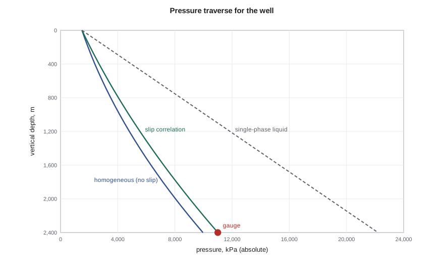
Ethan's result surprises him. Gravity accounts for about 96 percent of the pressure drop, friction for about 4 percent, and acceleration is negligible. 'That is typical of an oil well,' Marisol says. 'The fight is against the weight of the column, which is why holdup matters so much. Now compare the bottomhole pressure with the gauge.' The homogeneous model predicts about 9,960 kPa, while the gauge reads closer to 11,000 kPa. The difference is the holdup the model has ignored.
Gas wells and gathering lines
The balance of terms changes in other systems. In a gas well, the density is low, so the gravity term is small and friction dominates at high rates; at low rates, liquid held up in the tubing makes gravity grow again, which is the start of liquid loading. In a nearly horizontal gathering line, gravity contributes only on the uphill sections, so friction usually dominates on flat ground. On hilly terrain, though, the uphill sections can contribute a large elevation loss even when the net elevation change is small, because holdup on the uphills is high and on the downhills it is low, so the pressure lost climbing is not recovered descending. This is why the line profile matters as much as its length.
| System | Gravity | Friction | Acceleration |
|---|---|---|---|
| Oil well, moderate rate | 70 to 95% | 5 to 30% | under 1% |
| Gas well, high rate | 20 to 50% | 50 to 80% | up to a few % |
| Flat gathering line | under 10% | 90% or more | under 1% |
| Hilly gathering line, low rate | 50% or more | under 50% | under 1% |
Where the homogeneous model is still useful
Despite its limits, the homogeneous model is widely used. It provides quick screening, a sanity check on software output, and a basis for the friction term in some correlations. It is the standard approach for sizing short facility piping, relief and flare lines carrying two-phase fluid, and for critical-flow calculations through chokes and orifices. It also helps an engineer understand which term dominates before choosing a more detailed method: if friction dominates, small errors in holdup matter little; if gravity dominates, the holdup model becomes the most important choice.
A note on units and consistency
Multiphase calculations combine quantities from many sources: rates at standard conditions, volume factors, densities at line conditions, viscosities in centipoise, and pipe sizes in inches or millimetres. Most errors in hand calculations come from mixing standard and in-situ volumes or from forgetting to convert the gas rate to line conditions. A good habit is to convert everything to consistent SI units at the start, compute in-situ volumetric rates for each phase, and only then form superficial velocities. Ethan's script follows that pattern, converting to field units only for printing on the US site.
Worked problem
Gradient components in a gathering line segment
A 500 m uphill segment of the north pad line rises 10 m. The mixture velocity is 2.0 m/s, the no-slip density 300 kg/m³, the in-situ density from a slip correlation 520 kg/m³, the friction factor 0.020 and the diameter 0.154 m. Estimate the gravity and friction losses.
Show solution
- Gravity: ρ_s g Δz = 520 × 9.81 × 10 = 51.0 kPa.
- Friction: f ρ_n v_m² L / (2D) = 0.020 × 300 × 4.0 × 500 / (2 × 0.154) = 39.0 kPa.
- With the homogeneous density, gravity would be only 300 × 9.81 × 10 = 29.4 kPa.
Answer: About 90 kPa in total, with gravity the larger part; ignoring slip would understate the gravity loss by more than 40 percent.
Critical flow through chokes
One place where the homogeneous model is standard practice is the wellhead choke. When the pressure ratio across a choke falls below roughly 0.5 to 0.6, the mixture reaches its critical velocity in the choke throat, and the flow rate no longer depends on the downstream pressure. That is useful, because it isolates the well from pressure fluctuations in the gathering system: a slug arriving at the battery does not change the well's rate. Empirical choke equations, such as Gilbert's 1954 relation between wellhead pressure, liquid rate, gas-liquid ratio and choke size, and homogeneous critical-flow models such as Sachdeva's, are used to size chokes and to estimate rates when meters are unavailable.
For the gathering system designer, the choke defines the boundary between the well and the line. As long as each well flows through a critical choke, the line can be modelled with fixed inlet rates. When reservoir pressure falls and the chokes open fully, flow becomes subcritical, the wells start to feel the line pressure, and the well and line must be solved together with nodal analysis. Ethan notes that several of the older wells on the north pad are already fully open.
Common mistakes
MistakeUsing the no-slip density in the gravity term for slug flow.
InsteadUse the in-situ density from a holdup model; no-slip understates gravity.
MistakeAssuming elevation losses cancel on hilly terrain.
InsteadHoldup is higher uphill than downhill, so losses climbing are not recovered.
MistakeIncluding the acceleration term by default and then ignoring it in checks.
InsteadCompute E_k; neglect it only when it is small.
MistakeUsing standard-condition gas rates to compute velocities.
InsteadConvert to in-situ volumetric rates at line pressure and temperature first.
Summary and key terms
- The pressure gradient is the sum of gravity, friction and acceleration terms.
- The homogeneous model assumes no slip, so holdup equals the no-slip fraction.
- Mixture properties are volume-averaged with λ_L, and the friction factor comes from single-phase equations.
- Acceleration is usually negligible except at low pressure and high velocity.
- Calculations march along the pipe because properties change with pressure and temperature.
- Gravity dominates oil wells; friction dominates flat gathering lines and high-rate gas wells.
- Pressure gradient
- The rate of change of pressure with distance along the pipe.
- Homogeneous model
- A model that treats gas and liquid as moving together with no slip.
- Elevation gradient
- The pressure loss due to the weight of the fluid column.
- Acceleration gradient
- The pressure loss needed to speed up the expanding mixture.
- Marching calculation
- Step-by-step integration of the gradient along the pipe.
- Pressure traverse
- A plot of pressure against depth or distance along the flow path.
Practice problems
Work each problem on paper first, then reveal the answer to check.
What are the three components of the multiphase pressure gradient?
Show answer
Gravity (elevation), friction and acceleration.
When is the homogeneous model accurate?
Show answer
When slip is small, as in dispersed bubble or mist flow at high velocity.
Why do elevation losses on hilly terrain not cancel?
Show answer
Holdup is higher on the uphills than on the downhills.
What does E_k measure?
Show answer
The relative importance of the acceleration term; near 1 indicates near-critical flow.
Lesson quiz · 5 questions
Score 60% or more to complete this lesson.
Create a free account to save your progress, take quizzes and earn a certificate.