Flow patterns in horizontal and inclined pipes

Sofia takes Ethan to a pipe yard behind the Drayton Valley field office, where a short length of clear acrylic pipe from an old training rig has been mounted on a frame with a small pump and an air blower. Wes Brandt, the lease operator, runs water through it and slowly opens the air valve. At first the air rides along the top as a thin layer. Then small waves appear on the water surface, grow, and suddenly a wave fills the pipe and races along it as a plug of liquid. 'That is a slug,' Wes says. 'On the real line you cannot see it, but you can hear it hit the battery, and you can see it on the separator level controller.'

This lesson describes the flow patterns that form when gas and liquid flow together in horizontal and gently inclined pipes, explains the physical mechanisms that cause the transitions between them, and introduces flow pattern maps, the charts used to predict which pattern to expect for given rates, fluids and pipe sizes.

The main horizontal flow patterns

In a horizontal pipe gravity pulls the liquid to the bottom, so the patterns are not symmetric about the pipe axis as they are in vertical flow. Researchers name them in slightly different ways, but most descriptions recognize the following groups.

Stratified smooth flow occurs at low gas and liquid rates. The liquid runs along the bottom of the pipe with a smooth interface and the gas flows above it. As the gas rate increases, waves form on the interface, giving stratified wavy flow. Both are called segregated flow because the phases are separated.

Intermittent flow includes elongated bubble flow and slug flow. At moderate gas rates and higher liquid rates, waves grow until they bridge the pipe. Each bridge becomes a liquid slug that is pushed along by the gas behind it at about the mixture velocity or faster, picking up the slow liquid film ahead of it and shedding liquid from its tail. Between slugs, long gas bubbles ride over a liquid film. When the slugs contain few gas bubbles the pattern is often called plug or elongated bubble flow; when they are aerated and frothy it is called slug flow.

Annular flow occurs at high gas rates. The gas forms a fast core along the centre of the pipe, and the liquid forms a film around the wall, thicker at the bottom than at the top because of gravity, with some liquid carried as droplets in the core. At very high gas rates and low liquid rates the film may be almost entirely torn into droplets, giving mist flow.

Dispersed bubble flow occurs at high liquid rates. The turbulence of the liquid breaks the gas into small bubbles that are spread through the liquid, more concentrated near the top of the pipe at moderate rates and nearly uniform at high rates.

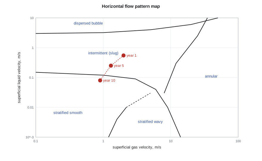
Why the transitions happen

The transition from stratified to slug flow is driven by interfacial waves. Gas flowing over a liquid surface lowers the pressure over a wave crest, much as air flowing over a wing creates lift. If the gas is fast enough, this suction overcomes gravity and the wave grows. Taitel and Dukler expressed this as a modified Kelvin-Helmholtz instability: a wave grows when the gas velocity exceeds a critical value that depends on the liquid level, the density difference and the pipe diameter. Once the wave grows to fill the pipe, it becomes a slug if there is enough liquid to keep it alive; otherwise the wave is torn into droplets and the flow becomes annular.

The transition to dispersed bubble flow happens when liquid turbulence is strong enough to break the gas into bubbles smaller than the size at which they would coalesce and rise to the top. The transition from stratified smooth to stratified wavy happens when the gas is fast enough to generate waves by wind shear. Each transition has its own physics, which is why mechanistic maps have several differently shaped boundaries rather than a single line.

Flow pattern maps

A flow pattern map is a chart, usually on logarithmic axes, with superficial gas velocity on one axis and superficial liquid velocity on the other. Regions of the chart correspond to patterns, and the boundaries between them are transition lines. The Mandhane map, published in 1974, was drawn from a large database of air-water and other experiments in horizontal pipes and is still useful for quick screening. Its boundaries are fixed, so it does not respond to changes in pipe size or fluid properties.

Mechanistic maps, such as the one developed by Taitel and Dukler in 1976, calculate the transition boundaries from physical models. Because the boundaries depend on pipe diameter, fluid densities, viscosities, surface tension and inclination, they move as conditions change. Commercial software draws these maps for each segment of a line. Empirical correlations such as Beggs and Brill use their own pattern definitions, based on a Froude number and the no-slip liquid fraction rather than on superficial velocities.

The Beggs-Brill pattern boundaries

Beggs and Brill, working with an inclinable test loop at the University of Tulsa in the early 1970s, classified horizontal flow into segregated, intermittent and distributed patterns, with a transition zone between segregated and intermittent. They placed the boundaries on a chart of mixture Froude number against no-slip liquid fraction:

The boundary lines are power-law functions of λ_L. Low Froude numbers, meaning slow flow in a large pipe, give segregated flow. High Froude numbers with little liquid give distributed (mist) flow, and the region between gives intermittent flow. Their holdup correlation, covered in lesson 7, uses different coefficients in each region.

# Beggs-Brill horizontal flow pattern boundaries (as given in the 1973 correlation and its later revision)
import math
SI = True   
g = 9.81
def pattern(vsl, vsg, D):
    vm = vsl + vsg
    lam = vsl / vm
    NFr = vm * vm / (g * D)
    L1 = 316 * lam ** 0.302
    L2 = 0.0009252 * lam ** -2.4684
    L3 = 0.10 * lam ** -1.4516
    L4 = 0.5 * lam ** -6.738
    if (lam < 0.01 and NFr < L1) or (lam >= 0.01 and NFr < L2): p = "segregated"
    elif lam >= 0.01 and L2 <= NFr <= L3: p = "transition"
    elif (0.01 <= lam < 0.4 and L3 < NFr <= L1) or (lam >= 0.4 and L3 < NFr <= L4): p = "intermittent"
    else: p = "distributed"
    return lam, NFr, p
D = 0.154
cases = [(0.05, 0.5), (0.05, 3.0), (0.20, 2.0), (0.50, 1.5), (1.50, 0.8), (0.10, 12.0)]
for vsl, vsg in cases:
    lam, NFr, p = pattern(vsl, vsg, D)
    if SI: print(f"vSL {vsl:4.2f} m/s, vSG {vsg:5.2f} m/s: lambda {lam:5.3f}, Froude {NFr:7.3f} -> {p}")
    else:  print(f"vSL {vsl * 3.2808:4.2f} ft/s, vSG {vsg * 3.2808:5.1f} ft/s: lambda {lam:5.3f}, Froude {NFr:7.3f} -> {p}")

vSL 0.05 m/s, vSG  0.50 m/s: lambda 0.091, Froude   0.200 -> segregated
vSL 0.05 m/s, vSG  3.00 m/s: lambda 0.016, Froude   6.158 -> segregated
vSL 0.20 m/s, vSG  2.00 m/s: lambda 0.091, Froude   3.204 -> transition
vSL 0.50 m/s, vSG  1.50 m/s: lambda 0.250, Froude   2.648 -> intermittent
vSL 1.50 m/s, vSG  0.80 m/s: lambda 0.652, Froude   3.502 -> intermittent
vSL 0.10 m/s, vSG 12.00 m/s: lambda 0.008, Froude  96.913 -> distributed

Ethan's six cases show how sensitive the pattern is to rates. A slow line with little liquid is segregated. Raising the liquid velocity at moderate gas velocity moves the flow into the transition zone and then into intermittent flow, while very high gas velocity with little liquid gives distributed flow. 'Look: our line in its first year sits right in the intermittent region,' Sofia says. 'By year ten, with half the gas and a third of the liquid, it will be segregated. Same pipe, different physics.'

Effect of inclination

Even small inclinations have a strong effect on gas-liquid flow. In an uphill section, gravity holds liquid back, so holdup rises sharply and the stratified region shrinks: a slope of only one or two degrees can turn stratified flow into slug flow at the same rates. In a downhill section, gravity accelerates the liquid, which runs faster than in a horizontal pipe, thins out and may remain stratified at gas and liquid rates that would slug in a horizontal line. Real gathering lines follow the terrain, so their segments alternate between uphill and downhill, and the flow pattern can change from one segment to the next.

The low points between a downhill and an uphill section are particularly important. Liquid collects there, especially at low gas velocities, and periodically the gas pushes the accumulated liquid over the next crest as a terrain slug. Terrain slugging is discussed in lesson 11. For flow pattern prediction, the practical rule is to check every uphill section separately, because the uphill segments usually set the holdup and the slug behaviour of the whole line.

Using flow patterns in design

Flow pattern prediction is not an end in itself. It tells the engineer which holdup and friction model to use, whether to expect slugs at the facility, and how the line will behave as rates change over field life. Designers generally try to avoid two situations: very slow stratified flow on uphill sections late in life, where liquid builds up and the gravity loss grows, and long-wavelength slug flow at a riser or facility inlet that the separators cannot absorb. Choosing a smaller diameter raises velocities and can keep the flow in a more stable, higher-holdup-sweeping regime, at the cost of more friction early in life. That trade-off is the core of lesson 12.

Limits of flow pattern maps

Flow pattern boundaries are not sharp lines. In experiments the transition between patterns occurs over a band of rates, and different observers can classify the same flow differently, especially near the slug-annular boundary. Most maps were developed with air and water at low pressure in pipes of 1 to 6 inches. Oil, high-pressure gas, larger diameters and long distances can all shift the boundaries. Treat a map as a guide to which physics dominates, not as a precise prediction, and look for field evidence such as separator level swings or pressure fluctuations to confirm the pattern in an operating line.

Three-phase flow: oil, water and gas

Most gathering lines in the Tamarack Lake field carry water as well as oil and gas, and the water cut rises over field life. In a horizontal pipe at low velocity, water and oil can themselves separate into layers, with water along the bottom, oil above it and gas on top. This matters for corrosion, because a continuous water layer wets the steel, and for pressure drop, because the liquid layers flow at different velocities. At higher velocities the turbulence mixes oil and water into a dispersion, which may be oil-continuous or water-continuous. The change from one to the other, called phase inversion, typically occurs somewhere between 30 and 70 percent water cut depending on the oil, and near inversion the effective viscosity of the mixture can rise sharply.

Most correlations treat oil and water as a single liquid with volume-averaged properties, which works reasonably well for pressure drop when the liquids are well mixed. Designers should still check whether water is likely to separate in slow, late-life flow, because a stratified water layer on uphill sections and in low spots is where internal corrosion and solids deposition usually begin. Ethan adds a line to his notes: at year ten, with a 70 percent water cut and a mixture velocity below 1 m/s (3 ft/s), the north pad line will probably run with free water along the bottom.