Production surveillance and the artificial lift plan: capstone

Ethan's rotation ends with an assignment from Marisol Vega: write the artificial lift plan for the 04-22 for its first ten years, and present it to the asset team. 'You have the inflow model, the tubing model, the nodal analysis and the lift screens,' she says. 'Now put them together with costs, a schedule and a surveillance plan, and tell us what to do and when. Show us what would change your mind.'

This capstone lesson covers production surveillance, the data that tell a production engineer how a well is behaving, the diagnosis of underperforming wells, decline analysis and forecasting, and the economic comparison of artificial lift plans over a well's life. It ends with Ethan's lift plan, which draws together every earlier lesson.

Production surveillance

Surveillance is the routine collection and review of the data that show how wells, lift systems and facilities are performing. Its purpose is to find problems early, while they are cheap to fix, and to find opportunities, wells that could produce more. Good surveillance is a habit: the same data, reviewed on the same schedule, against expected values, with exceptions acted on.

The main data sources are:

• Well tests, in which a well's flow is sent through a test separator for a set period to measure oil, water and gas rates. Tests are the basis of allocation, which assigns a battery's or pad's measured sales back to individual wells.

• Wellhead and casing pressures and temperatures, often recorded continuously by a SCADA system.

• Lift system data: dynamometer cards and pump-off controller data for rod pumps, injection rate and casing pressure for gas lift, motor current, intake pressure and temperature for ESPs, and plunger arrival times.

• Fluid levels from acoustic shots, which give pump submergence and estimates of bottomhole pressure.

• Downhole gauges, where installed, which give flowing bottomhole pressure directly.

• Fluid samples and analyses: water chemistry for scale, oil properties for paraffin, and solids.

• Failure records: every pump change, rod part, tubing leak or ESP failure, with its cause.

At Prairie Crest Energy Ltd., the the Drayton Valley field office reviews an exception report each morning. It flags wells whose latest test is more than 15 percent below the expected rate, rod pumps whose cards show fluid pound or gas interference, and wells whose casing pressure has risen. Wes Brandt checks the flagged wells on his route that day.

Diagnosing an underperforming well

When a well produces less than expected, the production engineer works through the system in order, using the pressure budget from the first lesson. The question is always where the lost pressure or lost rate is going.

1. Check the data. A bad test, a failed meter or a misallocated volume is the most common cause of an apparent drop. Retest before acting.

2. Check the surface. Has the flowline or separator pressure risen? Is a choke partly plugged? Is a valve closed? Surface problems are cheap to fix and often missed.

3. Check the lift. Is the pump pumped off, worn or gas locked? Is gas lift injecting at the right depth? Is the ESP running in its operating range?

4. Check the wellbore. Is there scale, paraffin, sand fill or a tubing leak? Is the well loading up with liquid?

5. Check the inflow. Has the reservoir pressure fallen faster than expected, or has skin increased from fines, scale or damage? Has a nearby well or a waterflood changed the drainage?

Each step uses tools from earlier lessons: nodal analysis separates inflow problems from outflow problems, dynamometer cards diagnose rod pumps, and fluid levels and pressures test the inflow. A well whose inflow is fine but whose outflow has deteriorated needs a workover or lift change; a well whose inflow has dropped may need stimulation or may simply be depleting as expected.

Decline analysis and forecasting

Lift plans need a forecast of rates over the well's life. For wells in tight reservoirs, rate-time decline analysis is the usual tool. The Arps decline equations describe the rate as a function of time with an initial rate, an initial decline rate and an exponent b:

With b = 0 the decline is exponential, with b = 1 harmonic, and between them hyperbolic. Multistage fractured horizontal wells often show b values above 1 in early life, while flow is linear and the well has not yet felt its boundaries. Forecasting such wells with a single hyperbolic curve over decades overstates reserves, so engineers switch to an exponential terminal decline, often at 5 to 10 percent per year, once the hyperbolic decline rate falls to that level. Rate-transient analysis, which uses both rate and flowing pressure, gives better estimates of reservoir properties and forecasts than rate alone.

The forecast also sets when each lift change is needed. The nodal analysis from lesson 6, repeated with the transient inflow from lesson 3 at each future date, shows when the well will stop flowing naturally, and the lift screens show which method can deliver the forecast rate at each stage.

Comparing lift plans

A lift plan is a sequence: for example, natural flow, then gas lift, then rod pump. Each plan is compared over the well's life on several measures:

• Recovered oil over the planning period, because a method that draws the well down further or sooner recovers more.

• Capital cost of equipment and installation, and the timing of that spending.

• Operating cost: power or gas, chemicals, maintenance and, especially, workovers to replace failed equipment. Run life is often the largest uncertainty.

• Deferred production while the well waits for a rig or for equipment.

• Net present value at the company's discount rate, which brings these together, and the lift cost per unit of oil.

• Fit with the facility: available gas for lift, power, compression and water handling.

# Capstone: compare artificial lift plans over the life of the new horizontal well (10 years, monthly steps)
SI = True   
if SI:   # 04-22 Cardium; oil in m3/d, money in Canadian dollars
    qi, Di, b, Dmin = 52.0, 0.10, 0.9, 0.08 / 12        # Arps hyperbolic with a terminal decline (per month)
    netback, wc0, wc1, dfac = 330.0, 0.21, 0.55, 1.0
    plans = {
      "A: flow, then rod pump from month 5":            [(5, "flow", 1.00, 0.00, 0), (120, "rod", 0.95, 2500, 180000)],
      "B: flow, gas lift to month 24, then rod pump":   [(5, "flow", 1.00, 0.00, 0), (24, "gas lift", 0.88, 4200, 140000), (120, "rod", 0.95, 2500, 180000)],
    }
    unit = "m3"; cur = "CAD"; fq = lambda x: f"{x:,.0f} m3"; rod_cap = 45.0
else:    # 4-22H Bakken; oil in STB/d, money in US dollars
    qi, Di, b, Dmin = 1050.0, 0.16, 1.2, 0.06 / 12
    netback, wc0, wc1, dfac = 40.0, 0.35, 0.65, 1.0
    plans = {
      "A: flow, gas lift to month 30, then rod pump":   [(5, "flow", 1.00, 0, 0), (30, "gas lift", 0.92, 6500, 250000), (120, "rod", 0.95, 4500, 420000)],
      "B: flow, ESP to month 30, then rod pump":        [(5, "flow", 1.00, 0, 0), (30, "ESP", 1.00, 9000, 380000), (120, "rod", 0.95, 4500, 420000)],
      "C: flow, then rod pump from month 5":            [(5, "flow", 1.00, 0, 0), (120, "rod", 0.95, 4500, 420000)],
    }
    unit = "STB"; cur = "USD"; fq = lambda x: f"{x:,.0f} STB"; rod_cap = 450.0
def potential(m):              # oil rate the reservoir can deliver if the well is pumped off (hyperbolic, then exponential)
    t = m - 0.5; D = Di / (1 + b * Di * t)
    if D > Dmin: return qi / (1 + b * Di * t) ** (1 / b)
    tsw = (Di / Dmin - 1) / (b * Di); qsw = qi / (1 + b * Di * tsw) ** (1 / b)
    import math; return qsw * math.exp(-Dmin * (t - tsw))
def run(stages, esp_life=18):
    oil = 0.0; npv = 0.0; cost = 0.0; i = 0
    for m in range(1, 121):
        while m > stages[i][0]: i += 1
        _, kind, eff, opex, capex = stages[i]
        if m == (stages[i - 1][0] + 1 if i > 0 else 1): cost += capex; npv -= capex / 1.1 ** ((m - 1) / 12)
        q = potential(m) * eff
        wc = wc0 + (wc1 - wc0) * m / 120
        if kind == "rod": q = min(q, rod_cap * (1 - wc))        # gross capacity of the chosen pump unit
        if kind == "ESP" and (m - 5) % esp_life == 0: cost += 120000; npv -= 120000 / 1.1 ** (m / 12)   # ESP replacement
        vol = q * 30.4; oil += vol; cost += opex
        npv += (vol * netback - opex) / 1.1 ** (m / 12)
    return oil, npv, cost
for name, st in plans.items():
    oil, npv, cost = run(st)
    print(f"{name:48s} oil {fq(oil):>14s}   lift cost {cost / oil:5.2f} {cur} per {unit}   NPV10 {npv / 1e6:6.2f} million {cur}")
if not SI:
    oil, npv, cost = run(plans["B: flow, ESP to month 30, then rod pump"], esp_life=12)
    print(f"sensitivity: plan B with a 12-month ESP run life instead of 18 -> NPV10 {npv / 1e6:6.2f} million {cur}")
else:
    oil, npv, cost = run([(3, "flow", 1.00, 0.00, 0), (120, "rod", 0.95, 2500, 180000)])
    print(f"sensitivity: plan A with the pump needed at month 3 instead of month 5 -> NPV10 {npv / 1e6:6.2f} million {cur}")

A: flow, then rod pump from month 5              oil      36,332 m3   lift cost 12.87 CAD per m3   NPV10   8.99 million CAD
B: flow, gas lift to month 24, then rod pump     oil      35,452 m3   lift cost 18.05 CAD per m3   NPV10   8.59 million CAD
sensitivity: plan A with the pump needed at month 3 instead of month 5 -> NPV10   8.93 million CAD

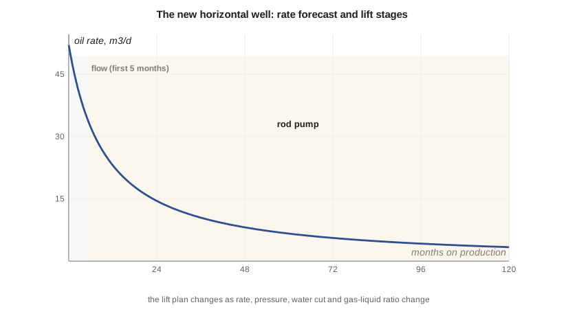
For the Cardium well, plan A, natural flow followed by a rod pump at month 5, recovers 36,332 m³ over ten years at a lift cost of 12.87 CAD per cubic metre and gives an NPV10 of 8.99 million CAD. Plan B, gas lift until month 24 and then a rod pump, recovers slightly less, 35,452 m³, because gas lift cannot draw the well down as far as a pump, and its lift cost is higher at 18.05 CAD per cubic metre because of compression and gas. Its NPV10 is 8.59 million CAD. The sensitivity shows that if the well needs the pump two months earlier than forecast, plan A still gives 8.93 million CAD. The recommendation is plan A: the rod pump is the cheaper, deeper-drawdown method for a well of this rate and depth.

The plan is robust because the difference in value between A and B, about 0.4 million CAD, is larger than any single sensitivity Ethan tested, and the rod pump suits a well that will settle at 10 to 20 m³/d for most of its life. The surveillance plan sets the trigger for installing the pump: when the flowing tests and the nodal analysis show the well cannot hold 25 m³/d against the current wellhead pressure, or when slugging begins, the pump goes in.

Presenting the plan

A lift plan is a recommendation for a decision, so its presentation should follow the decision. Ethan structures his in five parts:

1. The recommendation, in one sentence, with the expected value and recovery.

2. The basis: the inflow and tubing models, the forecast and how they were calibrated to the well's tests.

3. The alternatives and why they were not chosen, with the comparison table.

4. The uncertainties and their effect, shown as sensitivities, and what data would change the recommendation.

5. The actions and triggers: what equipment to order, when, and which surveillance measurements will tell the team when to switch lift.

Marisol's advice is to show the comparison and the sensitivities on one page each. Managers want to see that the alternatives were taken seriously and that the plan has clear decision points, not that every model detail is right.

Lift optimization over the field

One well's lift plan sits inside a field. Gas lift wells share a limited supply of injection gas, which should be allocated where it gives the most extra oil, using each well's gas lift performance curve: gas is moved to the well with the steepest slope until the slopes are equal. Rod pumps share workover rigs, which should go first to the failures losing the most oil. Pumping units can share power contracts, and ESPs can be scheduled to avoid peak power prices. Production engineers who manage a field use these allocation tools every week.

Run life is the single most important field-wide measure for artificial lift. Every failure costs a workover, deferred oil and sometimes a fishing job. Field teams track the mean time between failures for each lift type and well group, investigate every failure to find its root cause, and change practices that cause repeat failures: rod guides on deviated wells, better gas separation at the pump intake, scale inhibition, or different pump metallurgy.

What the production engineer brings together

This course has followed one well from its first test to a ten-year plan. Each lesson added one part of the system:

• The pressure budget in lesson 1 shows where the energy goes.

• Inflow performance in lessons 2 and 3 describes what the reservoir can deliver, and how it changes with time in tight, fractured wells.

• Tubing performance and multiphase flow in lesson 4, and liquid loading in gas wells in lesson 5, describe what the wellbore needs.

• Nodal analysis in lesson 6 joins inflow and outflow and shows when a well will stop flowing.

• Chokes and surface pressure in lesson 7 set the boundary at the top.

• Artificial lift in lessons 8 to 10 adds energy when the reservoir cannot lift the well.

• Facilities and emissions in lesson 11 decide what the surface can receive and how gas is handled.

• Surveillance and economics in this lesson turn the models into a plan and keep it current.

The production engineer's skill is in moving between these parts: seeing that a lost rate is a surface problem and not a reservoir problem, that a lift change needs compression or water handling, or that a cheaper plan carries a run-life risk that changes the decision.