
MEC-440 · Lesson 1 of 12 · 23 min
Energy systems and resources
In MEC-330 the engineers of Northgate District Energy in Winnipeg studied the cycles behind their plant: boilers, a back-pressure steam turbine, a possible gas turbine, chillers and heat pumps. In MEC-430 they designed the heating, ventilation and air conditioning of a new health centre that buys its heat and cooling from Northgate. Now the board has given them a larger question. Northgate has committed to stop burning fossil fuel for heat by 2040, and the board wants a plan: which energy sources and conversion technologies should supply the network, in what order, at what cost, and with what risks. Elena Varga leads the study. Graham Okoro, who knows the plant better than anyone, looks after the engineering of each option. Kofi Mensah, the energy consultant, builds the cost and carbon models. Tomás Reyes, now in his second year as an engineer in training, runs most of the calculations. Each lesson of this course looks at one family of energy conversion systems at the level of real plants and their economics, and asks what it could do for Northgate.
MEC-330 derived the ideal cycles. This course takes them as known and looks at what happens when the cycles become machines: the losses, the part-load behaviour, the auxiliaries, the cooling water, the emissions controls, the costs and the time it takes to build. It also widens the view to the conversion systems that are not heat engines at all, such as hydro turbines, wind turbines, solar cells, electrolysers, fuel cells and batteries. An engineer who plans an energy system has to compare all of them on a common footing, and that footing is the subject of this first lesson.
Primary energy, final energy and useful energy
Energy statistics distinguish three stages. Primary energy is the energy in a resource as found in nature: the chemical energy of natural gas, coal, oil and biomass, the nuclear energy in uranium, the kinetic energy of wind, the potential energy of water held behind a dam and the radiant energy of sunlight. Final energy is what consumers buy: electricity, natural gas, gasoline, district heat. Useful energy is what the consumer actually wants, such as heat in a room, motion of a vehicle or light. Every arrow from one stage to the next is a conversion, and every conversion has losses.
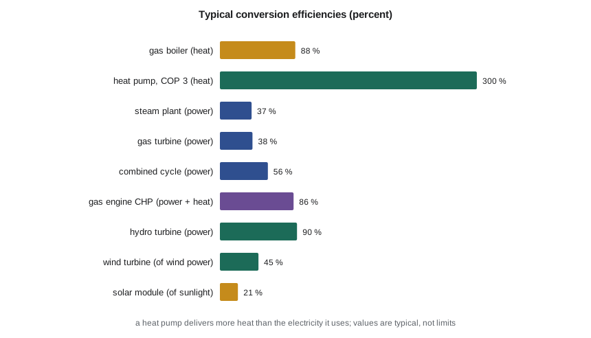
For fuels the accounting is straightforward: a gas boiler that is 88 percent efficient on the higher heating value turns 1 MWh of gas into 0.88 MWh of heat. For non-combustion sources the statistics need a convention. One common method counts the electricity from hydro, wind and solar as primary energy one for one; another credits it with the fuel a thermal plant would have needed to make the same electricity. The two methods can make the same country's energy supply look quite different, so when you read that a source supplies a certain share of primary energy, check which convention was used. For planning work it is safer to compare options on the final energy they deliver, on their emissions and on their cost, which is what this course will do.
Power and energy, capacity and capacity factor
Two numbers describe any plant. Its capacity, or power rating, in megawatts says how fast it can deliver energy. Its annual output, in megawatt-hours or gigawatt-hours, says how much it does deliver. The ratio of the actual annual output to what the plant would produce if it ran at full capacity all year is the capacity factor.
Capacity factors differ widely by technology and by the role a plant plays. Nuclear units typically run above 90 percent because their fuel is cheap and they are designed for steady output. Large hydro stations run at 50 to 70 percent depending on the water available. Wind farms on good sites reach 35 to 45 percent, solar farms in central Canada and the northern United States about 13 to 18 percent, and gas peaking turbines may run only a few hundred hours a year, a capacity factor of a few percent. A low capacity factor is not a failure. A peaking plant earns its keep by being available on the coldest or hottest afternoons, and a heating plant must be large enough for the coldest night of the decade even though that capacity is idle most of the year.
For a district heating network the same idea is called the load factor: annual heat delivered divided by peak demand times 8,760 hours. Northgate's network has a peak of 80 MW and sells 210 GWh of heat a year, a load factor of about 0.30. That one number will shape almost every decision in this course, because any plant with a high capital cost needs many running hours to pay for itself, and most of Northgate's capacity is needed for only a few weeks a year.
The electricity system behind the meter
Every electrified option Northgate considers, from heat pumps to electric boilers to electrolysers, depends on the grid it connects to, so the team starts by describing that grid. Across Canada, hydroelectric stations supply well over half of the electricity, nuclear plants in Ontario and New Brunswick supply roughly an eighth to a sixth, wind and solar together a little under a tenth, and fossil fuels, mainly natural gas, most of the rest. In 2024, a dry year in Quebec and Manitoba, hydro's share fell to about 55 percent. The mix varies enormously by province. Manitoba is one of the cleanest grids anywhere: hydro stations, mostly on the Nelson River in the north, produce more than 96 percent of its electricity, with wind and a small amount of natural gas making up the rest. Manitoba Hydro also exports large amounts of power to Saskatchewan, Ontario and the US Midwest, including Minnesota, over high-voltage lines.
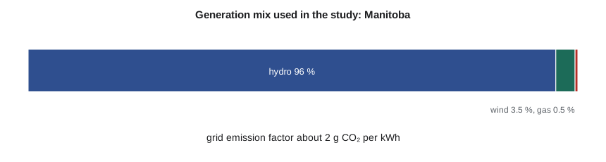
From the mix the team calculates a grid emission factor: the carbon dioxide emitted per kilowatt-hour generated, averaged over the year. The calculation multiplies each source's share by its direct stack emissions, about 1.0 kg/kWh for a coal plant, about 0.4 kg/kWh for a modern gas-fired combined cycle and zero for hydro, nuclear, wind and solar. Life-cycle emissions from building the plants and mining their fuel add a few to a few tens of grams per kilowatt-hour for the low-carbon sources, but they are small next to fuel combustion and the study leaves them out.
# Northgate District Energy: where the energy comes from today, and what the grid behind it looks like
SITE = 'ca'
# Generation shares (fractions) used in this study, rounded from recent national and state or provincial data
mix = {'ca': {'region': 'Manitoba', 'shares': {'hydro': 0.96, 'wind': 0.035, 'natural gas': 0.005}},
       'us': {'region': 'Minnesota', 'shares': {'coal': 0.20, 'natural gas': 0.26, 'nuclear': 0.20, 'wind': 0.27, 'solar': 0.05, 'hydro and other': 0.02}}}[SITE]
# Direct (stack) emission factors, kg CO2 per kWh generated, typical values
ef = {'coal': 1.00, 'natural gas': 0.40, 'nuclear': 0.0, 'wind': 0.0, 'solar': 0.0, 'hydro': 0.0, 'hydro and other': 0.0}
grid = sum(f*ef[k] for k, f in mix['shares'].items())
print(f"{mix['region']} generation mix used in the study:")
for k, f in mix['shares'].items():
    print(f"  {k:16s} {f*100:5.1f} %")
print(f"Generation-weighted direct emission factor: {grid:.3f} kg CO2/kWh")
# Northgate's own energy balance (same plant in both cities)
gas_GWh = 262.0            # natural gas burned per year (higher heating value)
heat_sold = 210.0          # heat delivered to customers, GWh
cool_sold = 32.0           # cooling delivered, GWh
elec_GWh = 9.5             # electricity bought for chillers, pumps and auxiliaries
gas_ef = 0.181             # kg CO2 per kWh of natural gas (HHV basis)
co2_gas = gas_GWh*1e6*gas_ef/1000      # tonnes
co2_el = elec_GWh*1e6*grid/1000
print(f"\nNorthgate today: gas {gas_GWh:.0f} GWh, electricity {elec_GWh:.1f} GWh")
print(f"  heat delivered {heat_sold:.0f} GWh, cooling {cool_sold:.0f} GWh")
print(f"  overall heat delivered per unit of fuel: {heat_sold/gas_GWh:.2f}")
print(f"  CO2 from gas {co2_gas:,.0f} t, from electricity {co2_el:,.0f} t, total {co2_gas+co2_el:,.0f} t per year")
print(f"  share of emissions from burning gas: {co2_gas/(co2_gas+co2_el)*100:.0f} %")
# Energy versus power: capacity factor of the peak boiler plant
peak_MW = 80.0
cf = heat_sold*1000/(peak_MW*8760)
print(f"\nPeak heat demand {peak_MW:.0f} MW; annual heat {heat_sold:.0f} GWh -> load factor {cf:.2f}")Manitoba generation mix used in the study: hydro 96.0 % wind 3.5 % natural gas 0.5 % Generation-weighted direct emission factor: 0.002 kg CO2/kWh Northgate today: gas 262 GWh, electricity 9.5 GWh heat delivered 210 GWh, cooling 32 GWh overall heat delivered per unit of fuel: 0.80 CO2 from gas 47,422 t, from electricity 19 t, total 47,441 t per year share of emissions from burning gas: 100 % Peak heat demand 80 MW; annual heat 210 GWh -> load factor 0.30
The result frames the whole study. On the Manitoba grid electricity carries almost no carbon, about 2 g/kWh, so almost all of Northgate's 47,000 t of annual emissions come from the gas it burns. Any option that replaces gas with grid electricity cuts emissions nearly to zero; the questions are cost, reliability and how much electricity the province can supply.
Average and marginal emissions
The average emission factor answers the question: what is the carbon content of a typical kilowatt-hour on this grid this year? A planner often needs a different number, the marginal emission factor: if Northgate adds 10 MW of electric load, which plants respond, and what do they emit? On most grids the marginal plant is a gas or coal unit, so the marginal factor can be two or three times the average. On a hydro grid that exports, the marginal effect of extra load is to export less, which raises emissions in the neighbouring grid that would have imported the power. Neither number is wrong; they answer different questions. Good studies state which one they use and test the conclusion with the other.
The same care applies to the future. A heat pump installed in 2028 will run until about 2050. What matters is the grid it will run on over those years, not the grid of the year it was bought. The team therefore uses a declining emission factor in its long-range model wherever policy makes a decline likely, and labels every such projection as a study assumption.
Energy security, reliability and the shape of demand
Carbon and cost are not the only criteria. A district heating utility in a city where winter nights reach thirty below must never fail. The team's evaluation therefore includes the reliability of each energy source on the coldest day, the redundancy of the plant, the ability to store fuel or heat, and the dependence on any single supplier, pipeline or transmission line. It also includes the shape of demand: Northgate's heat demand is highest exactly when solar output is lowest and when the grid itself is under most strain from electric heating across the region. Options that look fine on an annual energy balance can fail on that one cold, still, dark week.
| Criterion | What the team measures | Why it matters for Northgate |
|---|---|---|
| Cost | Levelized cost of heat over 25 years | Customers pay for the heat; the utility must stay competitive with building boilers |
| Carbon | Cumulative CO₂ to 2040 and annual CO₂ in 2040 | The board's 2040 commitment and the city's climate plan |
| Peak capability | Firm megawatts on the design day | Heat demand is greatest on the coldest night |
| Resilience | Redundancy, storage, fuel and grid dependence | Hospitals and housing rely on the network |
| Deliverability | Time to permit, build and connect | Plant must be in service before 2040 |
| Risk | Exposure to fuel prices, policy and technology | Decisions last 25 to 40 years |
Worked problem
Load factor and the cost of capacity
A 20 MW heat pump plant costs 40 million to build. If it supplies 100 GWh of heat a year, what is its capacity factor, and how much capital does each megawatt-hour carry if the capital is recovered at 7.1 percent of its cost each year? Repeat for a 40 MW plant of the same cost per megawatt that supplies 140 GWh.
Show solution
- 20 MW plant: \(\text{CF} = 100{,}000/(20 \times 8760) = 0.57\). Annual capital charge \(0.071 \times 40 = 2.84\) million, or \(2.84 \times 10^6/100{,}000 = 28.4\) per MWh.
- 40 MW plant: capital 80 million, \(\text{CF} = 140{,}000/(40 \times 8760) = 0.40\). Capital charge \(0.071 \times 80 = 5.68\) million, or 40.6 per MWh.
- Doubling the size added only 40 percent more heat, so each extra megawatt-hour carries much more capital.
Answer: The first 20 MW carries about 28 per MWh of capital; the second 20 MW about 70 per MWh of the extra heat it adds. High-capital plant belongs at the base of the load duration curve, where it runs many hours.
This simple calculation already hints at the shape of the final plan. Northgate's best strategy is unlikely to be a single technology sized for the peak. More likely it will combine a base-load plant with a high capital cost and low running cost, a mid-merit plant, storage to shave peaks, and a cheap, reliable peaking plant that runs only a few hundred hours a year. Lesson 4 will build the load duration curve that makes this precise.
How this course is organized
Lessons 2 and 3 look at thermal power plants, steam and gas turbine, as they are built and operated. Lesson 4 combines heat and power in cogeneration and district energy, the technology Northgate already uses. Lessons 5 to 8 cover renewable sources: hydro, wind, solar and the thermal renewables, geothermal and biomass. Lesson 9 is an overview of nuclear power, including the small modular reactors now under construction. Lessons 10 and 11 cover hydrogen and storage, the technologies that move energy in time and between sectors. Lesson 12 brings everything together in an economic comparison of pathways to 2040 and the team's recommendation to the board.
Common mistakes
MistakeComparing a wind farm and a gas plant on capacity alone.
InsteadCompare the energy delivered, the capacity available at peak and the cost per megawatt-hour.
MistakeUsing this year's grid emission factor for equipment that will run for 25 years.
InsteadUse a projection of the grid over the equipment's life, and state it as an assumption.
MistakeTreating a low capacity factor as a sign of a bad plant.
InsteadAsk what role the plant plays; peaking plant is valuable for its availability, not its hours.
MistakeMixing primary-energy conventions when comparing countries or sources.
InsteadCheck whether non-combustion electricity is counted one for one or by a fuel-equivalent method.
MistakeIgnoring the coldest week when an annual balance looks good.
InsteadCheck every option against the design day as well as the year.
Summary and key terms
- Primary energy is converted to final energy and then to useful energy, with losses at each step.
- Capacity factor is annual energy divided by rated power times 8,760 hours; it reflects both the technology and the plant's role.
- Northgate's network has an 80 MW peak, 210 GWh of annual heat and a load factor of about 0.30.
- The local grid is almost entirely hydro, at about 2 g CO₂ per kWh, so electrifying heat removes nearly all of Northgate's emissions.
- Average and marginal emission factors answer different questions; good studies state which they use.
- Options are judged on cost, carbon, peak capability, resilience, deliverability and risk.
- Primary energy
- Energy in a natural resource before conversion, such as the chemical energy of gas or the kinetic energy of wind.
- Final energy
- Energy delivered to and paid for by consumers, such as electricity, gas or district heat.
- Capacity factor
- Annual energy produced divided by the energy the plant would produce at full power all year.
- Load factor
- For a network, annual energy delivered divided by peak demand times the hours in a year.
- Grid emission factor
- Average carbon dioxide emitted per kilowatt-hour generated on a grid.
- Marginal emission factor
- Change in grid emissions per extra kilowatt-hour of demand, set by the plants that respond.
- Heat pump
- A machine that moves heat from a low-temperature source to a higher temperature using work, delivering more heat than the work it uses.
- Design day
- The coldest or hottest day for which plant capacity is sized.
Practice problems
Work each problem on paper first, then reveal the answer to check.
A 5 MW wind turbine produces 17,000 MWh in a year. What is its capacity factor?
Show answer
\(17{,}000/(5 \times 8760) = 0.39\).
A network has a 60 MW peak and a load factor of 0.32. How much heat does it deliver each year?
Show answer
\(0.32 \times 60 \times 8760 = 168{,}000\) MWh, or 168 GWh.
A grid is 40 percent coal at 1.0 kg/kWh, 30 percent gas at 0.4 kg/kWh and 30 percent zero-carbon. What is its emission factor?
Show answer
\(0.4 \times 1.0 + 0.3 \times 0.4 = 0.52\) kg/kWh.
Why might a planner use a marginal emission factor for a new electric boiler rather than the grid average?
Show answer
Because the new load is met by the plants that respond at the margin, often fossil-fired, whose emissions can be much higher than the average.
A boiler is 88 percent efficient on the higher heating value. How much gas does 210 GWh of heat need?
Show answer
\(210/0.88 = 239\) GWh of gas.
Lesson quiz · 5 questions
Score 60% or more to complete this lesson.
Create a free account to save your progress, take quizzes and earn a certificate.