
MEC-430 · Lesson 5 of 12 · 23 min
Cooling loads by the radiant time series method
Cooling loads are harder to calculate than heating loads because they are dynamic. The sun moves across the facades, people arrive and leave, lights switch on, and the outdoor temperature swings through the day. Worse, heat that enters a room does not immediately become a load on the cooling system. Some of it is absorbed by the floor, walls and furniture and released hours later. This lesson explains the distinction that every cooling load method rests on, introduces the radiant time series method that ASHRAE recommends for design calculations, and applies it to the health centre on a July design day.
Heat gain is not cooling load
Four rates must be kept apart. Heat gain is the rate at which energy enters or is generated within a space at a given moment: solar radiation through a window, heat from a person, power drawn by a computer. Cooling load is the rate at which heat must be removed from the room air to hold it at the setpoint. Heat extraction rate is what the cooling equipment actually removes, which differs from the cooling load when the room temperature is allowed to float. Coil load is the load on the cooling coil, which includes the room loads plus the outdoor air, fan heat and other system gains.
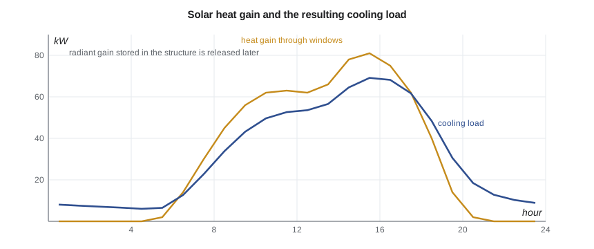
Heat gain becomes cooling load in two ways. The convective part of a gain warms the room air directly and becomes cooling load immediately. The radiant part travels as radiation to the room's surfaces, which absorb it and warm slowly; they then release it to the air by convection over the following hours. Solar radiation through windows is nearly all radiant, as is a large part of the heat from people and lights. The effect is that the peak cooling load is lower and later than the peak heat gain, by an amount that depends on the mass of the construction. A heavy concrete building smooths and delays its loads more than a light steel-framed one.
The radiant time series method
The radiant time series method, introduced by ASHRAE in the early 2000s as a simplification of the more rigorous heat balance method, handles the delay with two sets of coefficients. Conduction through walls and roofs is delayed by the mass of the assembly itself; the conduction time series, CTS, gives the fractions of a heat input at the outside surface that appear as heat gain at the inside surface in the current hour and each of the previous 23. Radiant heat gain inside the room is delayed by the room's mass; the radiant time series, RTS, gives the fractions of a radiant gain that become cooling load in the current hour and each of the previous 23. There are separate series for solar and non-solar radiant gains, and published sets for light, medium and heavy construction with different amounts of glass and carpet.
Each gain is split into its radiant and convective parts using recommended fractions: about 46 percent radiant for conduction through walls and roofs, about 60 percent of people's sensible heat, about 67 percent for typical lighting, and 10 to 30 percent for office equipment, depending on whether it has a fan. Transmitted solar radiation is treated as entirely radiant and uses the solar RTS. The convective parts become load in the same hour; the radiant parts are spread by the RTS. The cooling load for each hour is the sum.
The method assumes a design day that repeats: the same weather, sun and schedules every day, so that the gains from earlier hours that are still being released come from the same day's profile. That is why the series wrap around midnight. It is a method for the design peak, not for annual energy, which Lesson 11 covers.
The design day
For Winnipeg the July design day peaks at 30 °C with a daily range of about 11 K. The hourly outdoor temperatures come from ASHRAE's standard profile, which puts the minimum just before sunrise and the maximum at about 15:00 solar time. Solar irradiance on each facade comes from a clear-sky model and the sun's position for the site latitude on July 21. The program uses a simple clear-sky relation for teaching; design software uses ASHRAE's clear-sky model with optical depths published for each climate station. The window solar heat gain coefficient, 0.35, describes the fraction of incident solar radiation that ends up as heat inside, transmitted or absorbed and reradiated.
Opaque walls and the roof gain heat by conduction driven by the sol-air temperature, the outdoor temperature raised by the absorbed solar radiation. For the roof the effect is large: a dark roof in strong sun can reach a sol-air temperature 30 K above the air. The health centre's roof has a light-coloured membrane and is well insulated, so its conduction gain is small.
Here α is the surface's solar absorptance, \(E_t\) the total incident irradiance, \(h_o\) the outside surface coefficient, about 17 W/m²K, and the last term a small correction for long-wave exchange with the sky, about 4 K for a roof and zero for walls.
# Building cooling load by a simplified radiant time series (RTS) calculation, design day in July
import math
SITE = 'ca'
d = {'ca': dict(lat=49.9, tdb=30.0, rng=11.0), 'us': dict(lat=44.9, tdb=33.0, rng=10.5)}[SITE]
ti = 24.0
frac = [.82,.88,.92,.95,.98,1.0,.98,.91,.74,.55,.38,.23,.13,.05,0,0,.06,.14,.24,.39,.50,.59,.68,.75]  # profile, hours 1-24
tout = [d['tdb'] - f*d['rng'] for f in frac]
# illustrative series for a medium-weight building with carpet and about 35 % glass (fractions, sum = 1)
rts_nonsolar = [.49,.17,.09,.05,.03,.02,.02,.01,.01,.01,.01,.01,.01,.01,.01,.01,.01,.01,.01,.01,0,0,0,0]
rts_solar    = [.54,.16,.08,.04,.03,.02,.02,.01,.01,.01,.01,.01,.01,.01,.01,.01,.01,.01,.01,0,0,0,0,0]
cts_wall     = [.02,.08,.12,.12,.11,.09,.08,.07,.06,.05,.04,.03,.03,.02,.02,.02,.01,.01,.01,.01,0,0,0,0]
def sun(hour, lat=d['lat'], decl=20.4):              # solar time, degrees
    H = 15*(hour - 12); la, de, Hr = map(math.radians, (lat, decl, H))
    sb = math.sin(la)*math.sin(de) + math.cos(la)*math.cos(de)*math.cos(Hr)
    beta = math.asin(max(-1, min(1, sb)))
    if beta <= 0: return 0, 0
    cphi = (math.sin(beta)*math.sin(la) - math.sin(de))/(math.cos(beta)*math.cos(la))
    phi = math.degrees(math.acos(max(-1, min(1, cphi)))); phi = phi if H > 0 else -phi   # azimuth from south, west +
    return beta, phi
def irr(hour, facing):                               # incident beam + diffuse on a vertical surface, W/m2 (simple clear-sky model)
    beta, phi = sun(hour)
    if beta <= 0: return 0.0
    Ebn = 1080*math.exp(-0.18/math.sin(beta)); Ed = 0.12*Ebn
    ct = math.cos(beta)*math.cos(math.radians(phi - facing))
    return Ebn*max(0, ct) + Ed*(0.55 + 0.437*ct + 0.313*ct*ct if ct > -0.2 else 0.45)
facades = {'south': (0, 50*16.8), 'west': (90, 30*16.8), 'north': (180, 50*16.8), 'east': (-90, 30*16.8)}
wwr, Uw, Uwin, SHGC, Uroof, A_roof, alpha = 0.35, 0.21, 1.60, 0.35, 0.14, 1500, 0.6
area = 6000.0
people, lights, equip = 400, 6.0*area, 10.0*area           # W
sched = [0]*7 + [.3, .9] + [1]*8 + [.6, .2] + [0]*5         # occupied about 08:00 to 18:00, hours 1-24
sens_frac = [(people*75, 0.6), (lights, 0.67), (equip, 0.3)]   # (W at full use, radiant fraction)
def roll(series, inp, h):
    return sum(series[j]*inp[(h - j) % 24] for j in range(24))
win_solar, win_cond, wall_cond = [0]*24, [0]*24, [0]*24
for f, (az, A) in facades.items():
    for h in range(24):
        E = irr(h + 0.5, az)
        win_solar[h] += wwr*A*SHGC*E
        win_cond[h] += wwr*A*Uwin*(tout[h] - ti)
        wall_cond[h] += (1 - wwr)*A*Uw*(tout[h] + alpha*E/17 - ti)
roof_in = [A_roof*Uroof*(tout[h] + 0.9*800*max(0, math.sin(sun(h + 0.5)[0]))/17 - ti) for h in range(24)]
conduction = [wall_cond[h] + roof_in[h] for h in range(24)]
cond_cts = [roll(cts_wall, conduction, h) for h in range(24)]
load = []
for h in range(24):
    sol = roll(rts_solar, win_solar, h)
    conv_int = sum(W*sched[h]*(1 - rf) for W, rf in sens_frac)
    rad_int = sum(roll(rts_nonsolar, [W*sched[k]*rf for k in range(24)], h) for W, rf in sens_frac)
    cnd = 0.54*cond_cts[h] + roll(rts_nonsolar, [0.46*c for c in cond_cts], h) + win_cond[h]
    load.append((sol, conv_int + rad_int, cnd))
tot = [sum(x) for x in load]; pk = max(range(24), key=lambda h: tot[h])
print(f"Design day: {d['tdb']:.0f} C peak, {d['rng']:.1f} K range, latitude {d['lat']} N, July")
print("Hour  outdoor  solar  internal  conduction  total sensible (kW)")
for h in range(8, 21):
    s, i, c = load[h]
    print(f"{h+1:3d}   {tout[h]:5.1f}   {s/1000:5.0f}    {i/1000:5.0f}      {c/1000:5.1f}      {tot[h]/1000:6.0f}")
lat = people*55*sched[pk]
print(f"Peak space sensible {tot[pk]/1000:.0f} kW at hour {pk+1}; occupant latent {lat/1000:.0f} kW")
print(f"Instantaneous solar gain at that hour {win_solar[pk]/1000:.0f} kW vs RTS cooling load {load[pk][0]/1000:.0f} kW")
print(f"Space load density {(tot[pk] + lat)/area:.0f} W/m2")
doas_coil = {'ca': 197, 'us': 195}[SITE]                  # kW, from lesson 2
doas_sens = 1.21*4500*(ti - 10.0)/1000                    # sensible cooling the 10 C outdoor air delivers to the rooms
fcu = tot[pk]/1000 - doas_sens
fans = 0.04*(doas_coil + fcu)                             # fan and pump heat, pipe gains
plant = doas_coil + fcu + fans
print(f"DOAS air at 10 C meets {doas_sens:.0f} kW of space sensible load; fan coils take the remaining {fcu:.0f} kW")
print(f"Block plant cooling: DOAS coil {doas_coil} + fan coils {fcu:.0f} + fan, pump and pipe gains {fans:.0f} = {plant:.0f} kW ({plant/3.517:.0f} tons)")Design day: 30 C peak, 11.0 K range, latitude 49.9 N, July Hour outdoor solar internal conduction total sensible (kW) 9 21.9 61 92 -2.2 151 10 23.9 67 108 1.5 177 11 25.8 69 113 5.2 187 12 27.5 66 115 8.6 190 13 28.6 66 116 11.4 193 14 29.4 70 117 13.8 201 15 30.0 72 118 15.7 206 16 30.0 71 119 16.7 206 17 29.3 64 120 16.4 200 18 28.5 62 82 15.5 160 19 27.4 54 40 14.0 109 20 25.7 27 16 11.3 54 21 24.5 18 11 8.9 38 Peak space sensible 206 kW at hour 15; occupant latent 22 kW Instantaneous solar gain at that hour 81 kW vs RTS cooling load 72 kW Space load density 38 W/m2 DOAS air at 10 C meets 76 kW of space sensible load; fan coils take the remaining 130 kW Block plant cooling: DOAS coil 197 + fan coils 130 + fan, pump and pipe gains 13 = 340 kW (97 tons)
Reading the result
The peak space sensible cooling load is about 206 kW at 15:00 solar time. Internal gains, about 120 kW at the peak, are the largest part: people, lights and medical and office equipment in a busy clinic. Solar gain through the windows adds about 70 kW, and conduction through walls, roof and glass only 15 to 23 kW. The program also shows the effect of the radiant time series: at the peak hour the instantaneous solar gain through the windows is 81 kW, while the solar cooling load is 72 kW. The difference is stored in the floors and released in the evening, which is why the 19:00 load is still over 100 kW after most people have left.
Adding the occupants' latent load of 22 kW gives a space load of about 38 W per square metre of floor. That is far below the 85 to 90 W/m² rule of thumb used in Lesson 1. The rule of thumb is not wrong so much as general: it covers whole-building loads including outdoor air in buildings with more glass and less careful design. The program then builds the plant load. The dedicated outdoor air arrives at 10 °C and meets about 76 kW of the space sensible load; four-pipe fan coils meet the remaining 130 kW or so. Adding the outdoor air coil load from Lesson 2 and an allowance for fan heat, pump heat and pipe gains gives a block cooling load of about 340 kW, or 97 tons.
| Part of the load | kW at the block peak | Notes |
|---|---|---|
| Internal gains (sensible) | about 120 | people, lights, equipment |
| Solar through windows | about 66 to 72 | after the radiant time series |
| Conduction, walls, roof, glass | about 15 to 23 | small in a well-insulated building |
| Occupant latent | 22 | absorbed by the dry outdoor air |
| Outdoor air coil | about 195 to 197 | the largest single item |
| Fan, pump and pipe gains | about 13 | allowance |
| Block plant load | about 340 | compared with 510 to 540 by rule of thumb |
Block and peak loads
Each room's cooling load peaks at a different time. West rooms peak in the late afternoon, east rooms in the morning, interior rooms whenever they are busiest. Terminal units must be sized for each room's own peak, but the central equipment serving many rooms sees only the block load, the largest hourly sum, which is less than the sum of the room peaks. The ratio is the diversity of the load. For the health centre the sum of the individual room peaks, which Tomás will calculate at design development, is likely to be 15 to 20 percent above the block load. The fan coils are sized for room peaks; the energy transfer station's chilled water exchanger is sized for the block.
The design day also hides how rarely the peak occurs. A cooling plant sized for the design day runs near full output for perhaps a few dozen hours a year and below half output for most of its operating hours. That is the real argument for careful load calculation: every kilowatt of unnecessary capacity is a kilowatt that will spend its life running inefficiently at low load. Variable-speed fans and pumps and a heat exchanger connection to a district system tolerate part load far better than a small on-site chiller cycling on and off, which is one more reason the district connection suits this building.
Finally, the result must be checked against the shaded and unshaded cases. The program assumes no external shading. The architect has proposed fixed horizontal sunshades over the south windows and vertical fins on the west, which design software can model directly; on a south facade in July, a well-proportioned overhang can cut the transmitted solar gain by a third or more while hardly affecting winter sun, when the sun is low. Tomás reruns the calculation at design development with the shading included and reports the saving to the architect, because shading that pays for itself in smaller fan coils is easier to keep through value engineering.
Internal gains: the uncertain part
Internal gains are the most uncertain part of the calculation and the most important here. Lighting power is known from the lighting design. Occupancy can be estimated from the clinic schedule. Equipment power is the hard one. Nameplate ratings greatly overstate the heat actually given off, because equipment rarely draws its rated power, and measured values published by ASHRAE for office and medical equipment are far lower. Using nameplate data would roughly double the equipment load and oversize the cooling. Tomás uses 10 W/m², a value typical of measured clinic floors, and the imaging equipment's own data for the magnetic resonance and computed tomography rooms, which are handled by dedicated units.
Worked problem
Delayed solar load in one hour
A west window transmits solar heat gains of 2.0, 3.5 and 4.2 kW in the hours ending 14:00, 15:00 and 16:00, and the solar RTS begins 0.54, 0.16, 0.08. Ignoring earlier hours, estimate the solar cooling load at 16:00.
Show solution
- \(Q = 0.54 \times 4.2 + 0.16 \times 3.5 + 0.08 \times 2.0\).
- \(Q = 2.27 + 0.56 + 0.16 = 2.99\) kW.
Answer: About 3.0 kW of the 4.2 kW gain in the current hour is cooling load, plus smaller contributions from earlier hours not included here. The full calculation adds all 24 terms.
Common mistakes
MistakeTreating heat gain as cooling load.
InsteadSplit gains into convective and radiant parts and delay the radiant part.
MistakeUsing nameplate power for equipment gains.
InsteadUse measured heat gain values; nameplates overstate them greatly.
MistakeSizing central plant for the sum of room peaks.
InsteadSize central plant for the block load and terminals for room peaks.
MistakeForgetting the outdoor air coil when quoting the cooling load.
InsteadDistinguish space load from coil and plant load.
MistakeUsing the RTS method to estimate annual cooling energy.
InsteadUse it for design peaks; use simulation for energy.
Summary and key terms
- Heat gain, cooling load, heat extraction and coil load are different rates.
- Radiant gains are stored and released later, lowering and delaying the cooling load peak.
- RTS applies conduction and radiant time series to a repeating design day.
- The health centre's peak space sensible load is about 206 to 208 kW, mostly internal gains.
- The block plant load is about 340 kW, far below the rule-of-thumb estimate.
- Terminals are sized for room peaks and central plant for the block peak.
- Heat gain
- The rate at which heat enters or is generated within a space.
- Cooling load
- The rate at which heat must be removed from room air to hold the setpoint.
- Radiant time series
- Coefficients giving the fraction of a radiant heat gain that becomes cooling load in each subsequent hour.
- Conduction time series
- Coefficients giving the fraction of an outside heat input that appears as inside heat gain in each subsequent hour.
- Sol-air temperature
- The outdoor air temperature that would give the same heat flow into a surface as the actual combination of air temperature and solar radiation.
- Solar heat gain coefficient
- The fraction of incident solar radiation that enters through a window as heat.
- Block load
- The largest hourly total load for a group of spaces served by common equipment.
- Diversity
- The reduction from the sum of individual peaks to the peak of the total.
Practice problems
Work each problem on paper first, then reveal the answer to check.
A room has 2.0 kW of lighting gain, 67 percent radiant. How much becomes cooling load in the same hour if the first non-solar RTS coefficient is 0.49?
Show answer
Convective 0.66 kW plus \(0.49 \times 1.34 = 0.66\) kW radiant: about 1.32 kW.
A dark roof absorbs 0.9 of 900 W/m² with h_o = 17 W/m²K. Estimate the sol-air temperature rise, ignoring sky radiation.
Show answer
\(0.9 \times 900/17 = 48\) K.
Rooms with peaks of 12, 15 and 18 kW give a block peak of 38 kW. What is the diversity?
Show answer
\(38/45 = 0.84\).
In the program, what happens to the peak if the equipment density is 20 W/m² instead of 10?
Show answer
The internal gains rise by about 50 kW, and the peak sensible load to about 245 to 250 kW, depending on the radiant fraction.
Why does the 19:00 cooling load remain high after the clinics close?
Show answer
Solar and internal gains stored in the structure are still being released.
Lesson quiz · 5 questions
Score 60% or more to complete this lesson.
Create a free account to save your progress, take quizzes and earn a certificate.