
MEC-395 · Lesson 9 of 12 · 23 min
Temperature measurement
Temperature appears in three places on TL-3. The water temperature sets the density, viscosity and vapour pressure used in the test calculations. The bearing temperatures and the motor winding temperature are recorded in the mechanical run test that the customer has asked for, in which the pump runs for four hours at its rated point and the bearings must stabilize below a stated limit. And the ambient air temperature is logged because it affects the instruments themselves, as Lesson 4 showed. Temperature is easy to measure roughly and surprisingly hard to measure well, because a thermometer measures only its own temperature, and getting that to equal the temperature of interest is the real problem.
Temperature scales and standards
The kelvin is defined through the Boltzmann constant, and in practice temperatures are realized using the International Temperature Scale of 1990, ITS-90, which specifies fixed points, such as the triple point of water at 0.01 °C and the freezing points of several pure metals, and the instruments and equations used to interpolate between them. National metrology institutes realize the scale; calibration laboratories transfer it to working standards such as standard platinum resistance thermometers; and those calibrate industrial sensors, completing the traceability chain of Lesson 1. In a well-run test laboratory, every sensor's reading can be traced through this chain.
Resistance temperature detectors
A resistance temperature detector, or RTD, uses the steady increase of a metal's resistance with temperature. Platinum is the metal of choice because it is stable, resists corrosion and can be made very pure. The industrial standard, IEC 60751, defines the Pt100, an element of 100 Ω at 0 °C, whose resistance above 0 °C follows the Callendar–Van Dusen equation:
The sensitivity near room temperature is about 0.39 Ω per degree, so measuring temperature to 0.01 °C requires resistance to about 4 mΩ. The standard defines tolerance classes; class A, the grade used for TT-102, allows ±(0.15 + 0.002|t|) °C, and class B twice as much plus a little more. For the most accurate work an individual sensor is calibrated and its own coefficients used, which can reduce the uncertainty to a few hundredths of a degree.
Measuring an RTD's resistance means passing a current through it, and the connecting wires have resistance too. In a two-wire connection the lead resistance adds directly to the sensor's; the program shows that 15 m of ordinary 0.5 mm² cable adds over 1 Ω and an error of 2.7 °C. A three-wire connection uses a third lead to measure and subtract one lead's resistance, leaving only the mismatch between leads; with leads matched to 2 percent, the error falls to 0.03 °C. A four-wire connection passes the current through one pair of leads and measures the voltage through the other, which carries no current, so lead resistance does not enter at all. Test-grade RTDs on TL-3 are all four-wire.
The measuring current also heats the sensor. A 1 mA current in a Pt100 dissipates about 0.1 mW, and with the sensor in flowing water that raises its temperature by only a few thousandths of a degree. In still air, where heat escapes much less readily, self-heating can be ten or more times larger. Conditioners for RTDs use the smallest current consistent with low noise, often 1 mA or less.
# Temperature measurement on TL-3: the Pt100 RTD, lead resistance, a thermocouple and thermowell immersion
import math
A, B, R0 = 3.9083e-3, -5.775e-7, 100.0           # Callendar-Van Dusen coefficients (IEC 60751), t >= 0 C
def R_of_t(t): return R0*(1 + A*t + B*t*t)
def t_of_R(R): return (-A + math.sqrt(A*A - 4*B*(1 - R/R0)))/(2*B)
for t in (0.0, 20.0, 60.0, 100.0):
    print(f"Pt100 at {t:5.1f} C: {R_of_t(t):8.3f} ohm   (class A tolerance +/-{0.15 + 0.002*t:.2f} C, class B +/-{0.30 + 0.005*t:.2f} C)")
sens = (R_of_t(21) - R_of_t(19))/2
print(f"Sensitivity near 20 C: {sens:.4f} ohm per C")
# Lead resistance: 15 m of 0.5 mm2 copper per conductor
r_lead = 0.0175*15/0.5
R_meas = R_of_t(20.0)
print(f"\nEach lead {r_lead:.3f} ohm. Water truly at 20.000 C:")
print(f"  2-wire connection reads {t_of_R(R_meas + 2*r_lead):.3f} C (error {t_of_R(R_meas + 2*r_lead) - 20:+.3f} C)")
mismatch = 0.02                                   # 3-wire: lead resistances differ by 2 %
print(f"  3-wire with leads matched to 2 %: {t_of_R(R_meas + mismatch*r_lead):.3f} C (error {t_of_R(R_meas + mismatch*r_lead) - 20:+.3f} C)")
print(f"  4-wire: {t_of_R(R_meas):.3f} C (lead resistance does not enter)")
I, SH = 1.0e-3, 0.02                              # measuring current A, self-heating coefficient C per mW in flowing water
print(f"Self-heating at {I*1000:.0f} mA: {I*I*R_meas*1000:.3f} mW -> {SH*I*I*R_meas*1000:.4f} C")
# Type K thermocouple on the motor winding test, cold-junction compensation (linear approximation, about 41 uV/C near room temperature)
S = 41.0e-6
emf, t_cj = 2.300e-3, 24.0
print(f"\nThermocouple: emf {emf*1000:.3f} mV, cold junction at {t_cj:.1f} C -> hot junction about {t_cj + emf/S:.1f} C")
print(f"  if the cold junction were wrongly assumed to be 0 C: {emf/S:.1f} C (error {-t_cj:.1f} C)")
# Thermowell immersion: well as a fin, conduction to a pipe wall that is cooler than the water
k, Do, Di = 16.0, 0.010, 0.006                     # W/mK (stainless), well outside and inside diameters
print(f"\nThermowell immersion error (well treated as a fin, tip reading = fluid + (root - fluid)/cosh(mL)):")
for label, h, T_f, T_root in (('water, h 3000 W/m2K, 20 C, wall 17 C', 3000.0, 20.0, 17.0), ('air, h 40 W/m2K, 40 C, wall 25 C', 40.0, 40.0, 25.0)):
    m = math.sqrt(h*math.pi*Do/(k*math.pi*(Do*Do - Di*Di)/4))
    print(f"  {label}:")
    for L in (0.020, 0.060, 0.100):
        err = (T_root - T_f)/math.cosh(m*L)
print(f" immersion {L*1000:4.0f} mm ({L/Do:4.1f} diameters): error {err:+.4f} C")Pt100 at 0.0 C: 100.000 ohm (class A tolerance +/-0.15 C, class B +/-0.30 C)
Pt100 at 20.0 C: 107.793 ohm (class A tolerance +/-0.19 C, class B +/-0.40 C)
Pt100 at 60.0 C: 123.242 ohm (class A tolerance +/-0.27 C, class B +/-0.60 C)
Pt100 at 100.0 C: 138.505 ohm (class A tolerance +/-0.35 C, class B +/-0.80 C)
Sensitivity near 20 C: 0.3885 ohm per C
Each lead 0.525 ohm. Water truly at 20.000 C:
2-wire connection reads 22.704 C (error +2.704 C)
3-wire with leads matched to 2 %: 20.027 C (error +0.027 C)
4-wire: 20.000 C (lead resistance does not enter)
Self-heating at 1 mA: 0.108 mW -> 0.0022 C
Thermocouple: emf 2.300 mV, cold junction at 24.0 C -> hot junction about 80.1 C
if the cold junction were wrongly assumed to be 0 C: 56.1 C (error -24.0 C)
Thermowell immersion error (well treated as a fin, tip reading = fluid + (root - fluid)/cosh(mL)):
water, h 3000 W/m2K, 20 C, wall 17 C:
immersion 20 mm ( 2.0 diameters): error -0.0064 C
immersion 60 mm ( 6.0 diameters): error -0.0000 C
immersion 100 mm (10.0 diameters): error -0.0000 C
air, h 40 W/m2K, 40 C, wall 25 C:
immersion 20 mm ( 2.0 diameters): error -11.2857 C
immersion 60 mm ( 6.0 diameters): error -2.7755 C
immersion 100 mm (10.0 diameters): error -0.5758 CThermocouples
A thermocouple is two wires of different metals joined at the point of measurement. Because each metal develops a different thermoelectric voltage along a temperature gradient, the circuit produces a net voltage that depends on the temperatures of the measuring junction and of the reference junction, where the wires connect to copper. This is the Seebeck effect. The voltage is small, about 41 µV per degree for the common Type K (nickel-chromium and nickel-aluminium) near room temperature, and it is not linear; standard reference tables and polynomials, published internationally, relate voltage to temperature for each type.
Because the voltage depends on the temperature difference between the junctions, the reference junction temperature must be known. Historically it was held at 0 °C in an ice bath; modern instruments measure the temperature of the terminal block with a separate sensor and add the equivalent voltage, a technique called cold-junction compensation. The program, using a linear approximation of Type K's sensitivity, shows the scale of the issue: an emf of 2.300 mV with the junction box at 24 °C indicates about 80 °C, but if the compensation were missing or wrongly set the reading would be about 56 °C, 24 degrees low. Cold-junction errors are a common cause of thermocouples reading a few degrees wrong when terminal blocks warm up in the sun or near a drive.
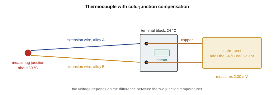
Between the measuring junction and the instrument, the circuit must continue in thermocouple wire, or in extension wire of matching thermoelectric properties, because any junction of dissimilar metals in a temperature gradient generates its own voltage. Copper wire from the sensor to a distant junction box, a common mistake, moves the reference junction to wherever the copper begins, at an unknown temperature. Thermocouples are less accurate than RTDs; standard-grade Type K wire is typically specified to about ±2 °C or a fraction of a percent of reading, whichever is larger. Their advantages are a very wide range, from cryogenic temperatures to well over 1,000 °C, small size, fast response and ruggedness, which is why the motor winding probes on TL-3 are thermocouples while the water temperature sensor is an RTD.
| Sensor | Typical range | Typical accuracy without individual calibration | Strengths | Limitations |
|---|---|---|---|---|
| Pt100 RTD, class A | −100 to 450 °C | ±0.15 °C at 0 °C, ±0.27 °C at 60 °C | Stable, accurate, standardized | Self-heating, slower, needs lead compensation |
| Type K thermocouple | −200 to 1,250 °C | About ±2 °C or a fraction of a percent of reading | Wide range, small, fast, rugged | Low output, needs cold-junction compensation |
| Thermistor | −50 to 150 °C | ±0.1 to 0.5 °C | Very sensitive, inexpensive | Nonlinear, narrow range |
| Infrared thermometer | −50 to over 1,000 °C | ±1 to 2 °C, plus emissivity effects | Non-contact, fast | Depends on surface emissivity and view |
Thermistors and infrared thermometers
A thermistor is a semiconductor resistor whose resistance falls steeply with temperature, typically by about 4 percent per degree near room temperature, ten times the relative sensitivity of platinum. Its relation to temperature is strongly nonlinear and is usually described by the Steinhart–Hart equation, \(1/T = a + b\ln R + c(\ln R)^3\) with T in kelvins. Thermistors are excellent for narrow ranges near room temperature, and they are used inside many instruments to measure the temperature of their own electronics for compensation, including the cold-junction sensors of thermocouple inputs.
An infrared thermometer measures the thermal radiation emitted by a surface, without contact. Every surface emits less than an ideal black body at the same temperature, by a factor called the emissivity, which ranges from about 0.95 for painted or oxidized surfaces to below 0.1 for polished metals. An infrared thermometer set for the wrong emissivity reads wrongly, and a shiny surface also reflects radiation from its surroundings. Lucie's group uses infrared thermometers for quick checks of bearing housings and motor frames, aiming at a spot of high-emissivity paint applied for the purpose, but never for test records.
Installation: making the sensor see the right temperature
Most temperature errors in practice are not sensor errors but installation errors. A sensor in a thermowell, a closed tube that protects it from the flow and lets it be removed without draining the pipe, is joined by the well's metal to the pipe wall. If the wall is at a different temperature from the fluid, heat flows along the well and the sensor reads somewhere between the two. The well behaves like a fin of the kind studied in heat transfer, and the error at the tip falls with the hyperbolic cosine of the immersion length times a parameter that grows with the heat transfer coefficient.
The program shows how strongly the error depends on the fluid. In water, where heat transfer from the fluid to the well is strong, a well immersed only two diameters reads within a hundredth of a degree even with the pipe wall three degrees cooler. In air, where heat transfer is roughly a hundred times weaker, the same well immersed two diameters reads more than 11 degrees low, and even ten diameters leaves an error of about half a degree. Rules of thumb for immersion, often quoted as ten or more well diameters for liquids and more for gases, are cautious for water and barely adequate for air.
Other installation effects follow the same logic. A sensor must be in good thermal contact with the well, often with a spring-loaded tip or heat-transfer paste. Surface sensors on bearing housings must be bonded or clamped and insulated from the surrounding air. Sensors measuring air temperature must be shielded from radiation from hot surfaces and from sunlight. And response time, the subject of Lesson 4, grows with every layer between the fluid and the element.
The bearing temperature run
For the mechanical run test, the TP-80's bearing housings carry four-wire Pt100 sensors in drilled holes reaching close to the outer races, held in place with spring-loaded fittings and covered with insulating caps. TT-401, from the control loop of MEC-390, measures oil sump temperature. The customer's specification limits the bearing temperature to 82 °C or a rise of 40 K above ambient, whichever is lower, once the temperatures have stabilized, which the specification defines as a change of less than 1 K over 30 minutes. Owen logs the sensors every 10 seconds, averages over 5-minute blocks, and computes the rate of change, so that the stabilization criterion is applied by the software rather than judged by eye.
Worked problem
Choosing a connection for the bearing RTDs
The bearing RTDs on the TP-80 are 8 m from the data acquisition cabinet, connected with 0.5 mm² copper. The test needs bearing temperatures to ±0.5 °C. Would a two-wire connection do?
Show solution
- Lead resistance: \(0.0175 \times 8/0.5 = 0.28\) Ω per conductor, 0.56 Ω for the loop.
- At 0.385 Ω per degree, 0.56 Ω corresponds to about 1.45 °C.
- Even with a fixed correction, the copper's resistance changes by about 0.4 percent per degree of cable temperature, adding drift of its own.
Answer: A two-wire connection would read about 1.5 °C high, three times the tolerance, and the error would drift with cable temperature. A three-wire connection would reduce it to a few hundredths of a degree; Owen uses four-wire sensors, which remove the question entirely.
Common mistakes
MistakeConnecting an RTD with two wires over a long run.
InsteadUse three-wire or, for test work, four-wire connections.
MistakeRunning copper wire from a thermocouple to a remote junction box.
InsteadUse matching extension wire all the way to the compensated terminals.
MistakeUsing an infrared thermometer on bare metal without considering emissivity.
InsteadMeasure a high-emissivity spot or use a contact sensor.
MistakeAssuming a short thermowell is adequate in gas or air.
InsteadImmersion error is far larger in gases; check it or immerse much deeper.
MistakeReading a temperature sensor before it has settled after installation.
InsteadAllow several time constants, as Lesson 4 showed.
Summary and key terms
- Temperatures trace to ITS-90 through calibrated working standards.
- A Pt100 follows the Callendar–Van Dusen equation, about 0.39 Ω per degree; class A allows ±(0.15 + 0.002|t|) °C.
- Two-wire RTD connections add lead resistance as error; three-wire leaves only the mismatch; four-wire removes it.
- Thermocouples measure a temperature difference and need cold-junction compensation and matching extension wire.
- Infrared readings depend on emissivity; thermistors are very sensitive but nonlinear.
- Thermowell conduction error is tiny in water but large in air, so immersion must suit the fluid.
- RTD
- A resistance temperature detector, using the change of a metal's resistance with temperature.
- Pt100
- A platinum RTD with a resistance of 100 Ω at 0 °C.
- Callendar–Van Dusen equation
- The standard relation between resistance and temperature for platinum RTDs.
- Four-wire connection
- An RTD connection with separate current and voltage leads, eliminating lead resistance.
- Thermocouple
- A pair of dissimilar wires joined at one end, producing a voltage that depends on temperature difference.
- Seebeck effect
- The generation of a voltage in a circuit of dissimilar conductors with junctions at different temperatures.
- Cold-junction compensation
- Measuring the reference junction temperature and correcting the thermocouple reading for it.
- Thermistor
- A semiconductor resistor whose resistance changes strongly with temperature.
- Emissivity
- The ratio of a surface's thermal radiation to that of a black body at the same temperature.
- Thermowell
- A closed tube inserted into a process that protects a temperature sensor.
Practice problems
Work each problem on paper first, then reveal the answer to check.
What is the resistance of a Pt100 at 40 °C?
Show answer
100(1 + 0.156332 − 0.000924) = 115.54 Ω.
A Pt100 reads 112.0 Ω. What temperature is that?
Show answer
About 30.9 °C.
In the program, what error would a two-wire connection give with 30 m leads of 1.0 mm² copper?
Show answer
Each lead 0.525 Ω, the same as the program's case, so about 2.7 °C.
A Type K thermocouple (about 41 µV/°C) gives 1.230 mV with the reference junction at 20 °C. Estimate the measured temperature.
Show answer
20 + 1.230/0.041 = 50 °C.
Why is the thermowell error so much smaller in water than in air?
Show answer
The heat transfer coefficient is far higher in water, so the well's tip is held close to the fluid temperature.
Lesson quiz · 5 questions
Score 60% or more to complete this lesson.
Create a free account to save your progress, take quizzes and earn a certificate.