
MEC-395 · Lesson 4 of 12 · 22 min
Static and dynamic characteristics of instruments
An instrument's datasheet is a compressed description of how it behaves, and reading one properly is a skill. The front page usually gives a single accuracy figure; the small print gives the nonlinearity, hysteresis, repeatability, temperature effects, long-term stability and response time that together make up that figure, and the conditions under which it holds. Owen's next task is to choose a pressure transducer for a new measurement Farah Siddiqui has asked for: the pressure pulsation at the TP-80's discharge, which tells the design group how strongly the impeller vanes interact with the volute. That task needs both halves of this lesson. Static characteristics describe an instrument's behaviour when the measurand is steady; dynamic characteristics describe how it follows a measurand that changes.
Static characteristics
The static calibration of Lesson 1 already introduced several static characteristics. The calibration curve relates output to input under steady conditions. Its slope is the static sensitivity. Its departure from a straight line is the nonlinearity, which may be quoted against a best-fit straight line, as in Lesson 1, or against the terminal line joining the ends of the range, which gives a larger number for the same instrument. Datasheets do not always say which, and the difference can be a factor of two, so Owen always checks the definition before comparing two products. Hysteresis is the difference between rising and falling readings. Repeatability is the scatter of repeated readings of the same input. Many manufacturers combine nonlinearity, hysteresis and repeatability into a single figure, often abbreviated NLHR, which is the best accuracy the instrument can offer at its reference temperature.
Instruments are also sensitive to their environment. A pressure transducer's zero and span shift with temperature; a typical specification might read ±0.015 percent of span per °C for zero and ±0.01 percent of reading per °C for span, outside a compensated range. If such a transducer is calibrated at 20 °C but its zero is not compensated, a test cell that warms to 32 °C on a summer afternoon shifts it by 12 × 0.015 = 0.18 percent of span, several times its NLHR figure; good transducers are compensated over a stated band, and the effect applies outside it. Supply voltage, mounting orientation, vibration and electromagnetic interference all have effects of their own, and a full datasheet lists them. Long-term stability, or drift, is the change over months, usually given as a percentage of span per year, and it is what the calibration interval of Lesson 1 guards against.
| Characteristic | Typical specification for a test transducer | What it means at 6 bar span |
|---|---|---|
| Nonlinearity, hysteresis and repeatability | ±0.04 % of span | ±2.4 mbar |
| Zero temperature effect | ±0.015 % of span per °C outside 15 to 25 °C | ±0.9 mbar per °C |
| Span temperature effect | ±0.01 % of reading per °C outside 15 to 25 °C | ±0.3 mbar per °C at 3 bar |
| Long-term stability | ±0.05 % of span per year | ±3 mbar per year |
| Response time | under 1 ms | irrelevant for steady tests |
| Overpressure limit | 2 × span without damage | 12 bar |
Two more static ideas complete the picture. Dead band, or threshold, is the range over which the input can change without any change in output, important in mechanical instruments with friction. Loading is the change a measuring instrument makes to the quantity it measures. Every instrument extracts some energy from the system: a thermometer takes heat from the water, a voltmeter draws current, an insertion flow probe disturbs the flow. Good instruments make that effect negligible. A data acquisition input with 1 MΩ impedance reading a strain-gauge bridge of 350 Ω source resistance loads it by about 0.035 percent, which is negligible; the same input reading a thermistor of 100 kΩ would load it by 9 percent, which is not.
Why dynamics matter
No instrument responds instantly. A thermometer must warm up to the temperature of the water around it; a pressure transducer's diaphragm has mass and must be accelerated; the fluid in a tube between a pressure tapping and a transducer must be pushed back and forth. When the measurand is steady, these effects do not matter: wait long enough and the reading settles. When the measurand changes, the reading lags behind it, or overshoots, or exaggerates some frequencies and suppresses others. The same mathematics that MEC-390 used for control systems describes instruments: most behave as zero-, first- or second-order systems.
A zero-order instrument has output proportional to input at all frequencies, with no lag. A potentiometer used to measure position is nearly zero order, as is a strain gauge, since the resistance changes as fast as the strain does. Real instruments approximate zero order only below some frequency, but for many purposes that is enough.
First-order instruments
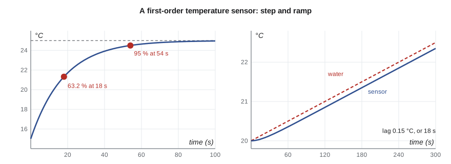
A temperature sensor in a thermowell is the classic first-order instrument. Heat flows from the water through the well and into the sensing element at a rate proportional to the temperature difference, and the element stores heat in its mass. The result is the first-order equation \(\tau\,dT_m/dt + T_m = T\), where \(T_m\) is the measured and T the true temperature, and τ is the time constant, the product of the sensor's thermal capacitance and the resistance to heat flow into it.
After a step change, the reading follows \(T_m = T_0 + \Delta T(1 - e^{-t/\tau})\): 63.2 percent of the change after one time constant, 95 percent after three and 99 percent after about 4.6. A sensor with a long time constant is not inaccurate in steady conditions, but readings taken before it has settled are wrong. On TL-3, Gilles found TT-102's time constant by a plunge test, moving the probe quickly from a bath at one temperature to another, and measured τ = 18 s.
A ramp input reveals a subtler error. When the water temperature rises steadily at rate R, the reading settles into following it at the same rate but with a constant lag of \(\tau R\) in temperature, or τ in time. TL-3's water warms by about half a degree a minute during long tests because the pump's losses heat it. The reading of TT-102 then lags the water by \(18 \times 0.5/60 = 0.15\) °C, the same size as the sensor's whole calibration tolerance. For the efficiency calculation that is harmless, since Lesson 3 showed density hardly matters; for a test of bearing temperature rise, where differences of a few tenths of a degree are reported, Owen allows for it.
Second-order instruments
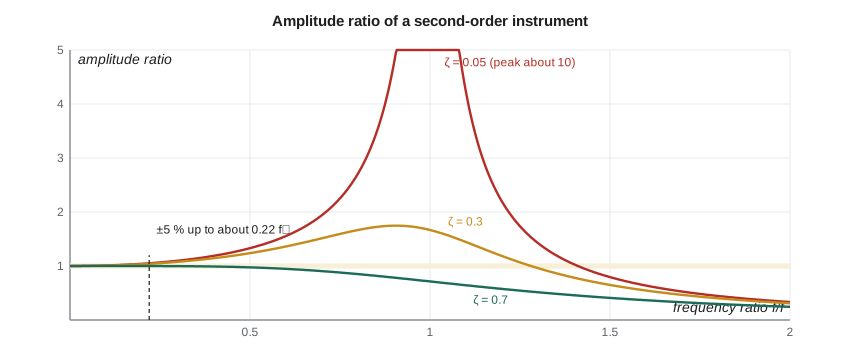
Instruments with an elastic element and mass, such as a diaphragm pressure transducer, an accelerometer or a load cell, behave as second-order systems, described by a natural frequency \(\omega_n\) and a damping ratio ζ. Their response to a sinusoidal input at frequency ω has an amplitude ratio
and a phase lag \(\phi = \arctan\big(2\zeta r/(1 - r^2)\big)\). Well below the natural frequency the amplitude ratio is close to one; near it, a lightly damped instrument exaggerates the input enormously; well above it, the instrument cannot follow at all. An instrument used for dynamic measurement must therefore have a natural frequency well above the highest frequency of interest. For light damping the amplitude error stays within 5 percent up to about a fifth of the natural frequency, a figure worth remembering. Damping of about 0.6 to 0.7 extends the flat range further and gives nearly linear phase, which is why some instruments are deliberately damped to that level.
A transducer's own natural frequency is often very high: tens of kilohertz for a stiff piezoresistive pressure sensor. But the installation can lower it drastically. A transducer mounted at the end of a length of tubing, with a small cavity in front of its diaphragm, forms a new second-order system: the liquid in the tube is the mass, the compliance of the cavity and any trapped air is the spring, and the natural frequency may fall to a few hundred hertz. Trapped air bubbles lower it further and add uncertainty. For steady measurements this does not matter, and the tubing even helps by smoothing the reading, but for pulsation it is decisive.
# Dynamic response of two TL-3 sensors: a first-order temperature probe and a second-order pressure transducer
import math
# 1. TT-102 in its thermowell behaves as first order with time constant tau (found from a plunge test)
tau = 18.0                                  # s
for frac in (0.632, 0.95, 0.99):
    print(f"Step test: {100*frac:4.1f} % of the change reached after {-tau*math.log(1 - frac):5.1f} s")
rate = 0.5/60                               # water warming at 0.5 deg C per minute, in deg C per second
print(f"Ramp of 0.5 C/min: steady lag tau x rate = {tau*rate:.2f} C (reading always behind the water)")
# Simulate the ramp to confirm, Euler steps of 0.01 s
T_true, T_read, dt = 20.0, 20.0, 0.01
for k in range(int(300/dt)):
    T_true += rate*dt; T_read += dt*(T_true - T_read)/tau
print(f"After 300 s: water {T_true:.3f} C, probe {T_read:.3f} C, lag {T_true - T_read:.3f} C")

# 2. Pressure pulsation: second-order transducer, amplitude ratio and phase versus frequency
def response(f, fn, zeta):
    r = f/fn; mag = 1/math.sqrt((1 - r*r)**2 + (2*zeta*r)**2)
    ph = -math.degrees(math.atan2(2*zeta*r, 1 - r*r)); return mag, ph
setups = [('on 1.2 m impulse line', 320.0, 0.08), ('close-coupled on 0.1 m nipple', 2400.0, 0.06), ('flush-mounted', 25000.0, 0.03)]
f_vp = 6*1760/60                            # vane-pass frequency, 6 vanes at 1,760 rpm
print(f"\nVane-pass frequency {f_vp:.0f} Hz and its second harmonic {2*f_vp:.0f} Hz")
print("  installation                      fn (Hz)  zeta   amplitude ratio at 176 / 352 Hz   phase at 176 Hz")
for name, fn, z in setups:
    m1, p1 = response(f_vp, fn, z); m2, _ = response(2*f_vp, fn, z)
    print(f"  {name:32s} {fn:7.0f}  {z:4.2f}      {m1:5.3f} / {m2:5.3f}                {p1:7.1f} deg")
# Highest frequency measured within +/-5 % amplitude error for each installation
for name, fn, z in setups:
    f = 0.0
    while abs(response(f + 1, fn, z)[0] - 1) <= 0.05: f += 1
print(f" {name}: flat within 5 % up to {f:.0f} Hz ({f/fn:.2f} fn)")Step test: 63.2 % of the change reached after 18.0 s Step test: 95.0 % of the change reached after 53.9 s Step test: 99.0 % of the change reached after 82.9 s Ramp of 0.5 C/min: steady lag tau x rate = 0.15 C (reading always behind the water) After 300 s: water 22.500 C, probe 22.350 C, lag 0.150 C Vane-pass frequency 176 Hz and its second harmonic 352 Hz installation fn (Hz) zeta amplitude ratio at 176 / 352 Hz phase at 176 Hz on 1.2 m impulse line 320 0.08 1.422 / 3.650 -7.2 deg close-coupled on 0.1 m nipple 2400 0.06 1.005 / 1.022 -0.5 deg flush-mounted 25000 0.03 1.000 / 1.000 -0.0 deg on 1.2 m impulse line: flat within 5 % up to 70 Hz (0.22 fn) close-coupled on 0.1 m nipple: flat within 5 % up to 525 Hz (0.22 fn) flush-mounted: flat within 5 % up to 5460 Hz (0.22 fn)
Measuring pressure pulsation
The TP-80 impeller has six vanes and runs at 1,760 rpm, so each vane passes the volute tongue 176 times a second, and the discharge pressure pulses at 176 Hz with harmonics at 352 Hz and above. Owen first considers using PT-210 itself. It sits on a 1.2 m impulse line, and a tap test, in which Gilles taps the line sharply and records the ringing, shows that installation has a natural frequency of about 320 Hz and a damping ratio of about 0.08. The program shows the consequence. At 176 Hz the amplitude ratio is 1.42, so the pulsation would be reported 42 percent too large; at the second harmonic, close to resonance, the error is a factor of 3.65. The record would be dominated by the measuring system, not the pump.
Close-coupling a transducer on a short nipple raises the natural frequency to about 2.4 kHz, and the error at 176 Hz falls to half a percent; it remains within 5 percent up to about 525 Hz. A flush-mounted transducer, its diaphragm level with the pipe wall, has the sensor's own natural frequency, about 25 kHz, and is flat to over 5 kHz. Owen specifies a flush-mounted piezoresistive transducer for Farah's pulsation test, fitted in a spare tapping close to the discharge flange, and leaves PT-210 on its impulse line for the steady head measurement, where the tubing's smoothing is an advantage.
Worked problem
Is the speed reading fast enough?
During a start-up test Owen wants to record the pump accelerating from rest to 1,760 rpm in 2.0 s, approximately linearly. The speed transmitter's output is filtered with a first-order time constant of 0.10 s. How far behind the true speed will its reading be during the acceleration?
Show solution
- The acceleration is a ramp at \(R = 1760/2.0 = 880\) rpm/s.
- After a few time constants the lag is \(\tau R = 0.10 \times 880 = 88\) rpm, or a delay of 0.10 s.
- At the end of the ramp the reading approaches the final speed with the same time constant.
Answer: The reading trails the true speed by about 88 rpm, five percent of rated speed. For a start-up record that is acceptable if the 0.1 s delay is stated; for anything finer the filter should be shortened.
Choosing an instrument
Selecting an instrument means matching both kinds of characteristic to the measurement. The range should cover the expected values with margin for transients but not so much that a specification stated as a percentage of span becomes poor at the working point; the overpressure rating should cover the worst event, such as the water hammer of a sudden valve closure. The static accuracy, including temperature and stability effects over the calibration interval, should fit the uncertainty budget. The dynamic response should be flat to well above the highest frequency of interest, or deliberately slow if a steady average is wanted. And the installation, which can spoil an excellent instrument, must be designed with as much care as the instrument is chosen.
Common mistakes
MistakeComparing two nonlinearity figures without checking their definitions.
InsteadBest-fit and terminal-line nonlinearity differ; compare like with like.
MistakeIgnoring temperature effects because the reference accuracy looks good.
InsteadAdd zero and span temperature effects for the conditions the instrument will actually see.
MistakeReading a first-order sensor before it has settled after a change.
InsteadWait about five time constants, or correct for the lag.
MistakeMeasuring pulsation through a long impulse line.
InsteadThe tubing forms a resonant system; close-couple or flush-mount the transducer.
MistakeAssuming a transducer's datasheet natural frequency applies to the installed sensor.
InsteadTubing, cavities and trapped air can lower it by orders of magnitude; test the installation.
Summary and key terms
- Static characteristics include sensitivity, nonlinearity, hysteresis, repeatability, temperature effects, drift, dead band and loading.
- A first-order sensor reaches 63.2 percent of a step in one time constant and lags a ramp by τR.
- TT-102 has τ = 18 s and lags the warming water by 0.15 °C.
- A second-order instrument is flat within 5 percent only up to about a fifth of its natural frequency when lightly damped.
- PT-210 on its impulse line would overstate the 176 Hz vane-pass pulsation by 42 percent.
- A flush-mounted transducer, flat to over 5 kHz, is used for pulsation; PT-210 stays for steady head.
- Static sensitivity
- The slope of the calibration curve; output change per unit input under steady conditions.
- Nonlinearity
- The departure of the calibration curve from a stated straight line.
- Drift
- Slow change of an instrument's output over time with constant input.
- Dead band
- The range through which an input can vary without changing the output.
- Loading
- The change an instrument causes in the quantity it measures.
- Time constant
- The time for a first-order system to reach 63.2 percent of a step change.
- Natural frequency
- The frequency at which an undamped second-order instrument would oscillate freely.
- Damping ratio
- The parameter that sets how strongly a second-order instrument resonates.
- Amplitude ratio
- The ratio of output to input amplitude for a sinusoidal input.
- Flush mounting
- Installing a pressure sensor with its diaphragm level with the wall, avoiding tubing resonance.
Practice problems
Work each problem on paper first, then reveal the answer to check.
A thermocouple has τ = 4 s. How long after a step does it read within 1 percent of the final change?
Show answer
4.6τ = 18 s.
A sensor with τ = 30 s measures a temperature rising at 2 °C per minute. What is the steady lag?
Show answer
30 × 2/60 = 1.0 °C.
A transducer installation has fn = 800 Hz and light damping. Up to what frequency is it flat within 5 percent?
Show answer
About 0.22 × 800 ≈ 175 Hz.
In the program, what amplitude ratio does the impulse-line installation give at 30 Hz?
Show answer
About 1.009, under 1 percent error, so steady and slowly varying pressures are measured well.
Why can a long impulse line be an advantage for a steady head measurement?
Show answer
It smooths rapid fluctuations, giving a steadier reading of the mean pressure.
Lesson quiz · 5 questions
Score 60% or more to complete this lesson.
Create a free account to save your progress, take quizzes and earn a certificate.