
MEC-395 · Lesson 2 of 12 · 23 min
Statistics of measurement data
With the instruments calibrated, Owen runs TL-3 at the TP-80's guarantee point and watches the flow reading on the screen. It does not sit still. It wanders between about 89.9 and 90.3 m³/h, with the occasional larger jump. Every measurement of a real quantity behaves like this, because the quantity itself fluctuates and because every instrument adds noise of its own. The question is not how to make the scatter vanish, which is impossible, but how to describe it, how to get the best value from it, and how to say how far that value can be trusted. Those are questions of statistics, and this lesson applies the tools of STAT-235 to measurement data.
Samples, populations and the shape of scatter
When Owen logs twenty readings of flow, he is taking a sample from a population: the infinite set of readings that the same measurement process would produce if it ran forever under the same conditions. The population has a true mean μ and a true standard deviation σ, which he can never know exactly. The sample gives estimates of both. The sample mean is
and the sample standard deviation, which estimates σ, is
The divisor \(n - 1\) rather than n corrects for the fact that the deviations are measured from the sample mean, which is itself fitted to the data; using n would underestimate σ on average. The quantity \(n - 1\) is the number of degrees of freedom, a term that will appear again whenever uncertainty is estimated from data.
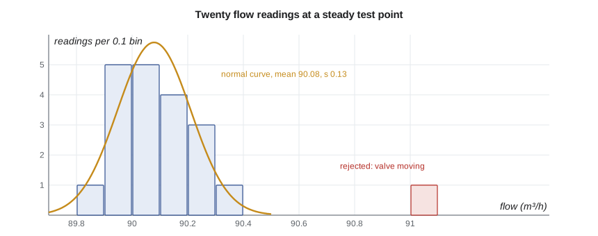
A histogram of many readings of a steady quantity usually has the bell shape of the normal, or Gaussian, distribution. This is not a coincidence. When an error is the sum of many small, independent contributions, none of which dominates, the central limit theorem says the sum tends to a normal distribution whatever the shapes of the individual contributions. Turbulent velocity fluctuations, electronic noise and small vibrations add up in exactly this way. For a normal distribution, about 68.3 percent of values lie within one standard deviation of the mean, 95.4 percent within two, and 99.7 percent within three; exactly 95 percent lie within 1.960 standard deviations.
How good is the mean?
The average of n readings is far more reliable than any one of them. If the readings are independent, the standard deviation of their mean, called the standard error, is
Averaging four readings halves the scatter of the result; averaging a hundred reduces it tenfold. This square-root law is the reason test standards ask for a number of readings at each test point, and the reason a data acquisition system that samples quickly and averages can give steadier results than a single reading. The law has a limit that is easy to forget: it reduces random error only. A flowmeter that reads 0.3 percent high still reads 0.3 percent high after a million readings are averaged.
The square-root law also assumes the readings are independent. Readings taken a few milliseconds apart from a slowly wandering quantity are not: each one is close to the last, and averaging a thousand of them in one second is not a thousand independent pieces of information. The flow in TL-3 wanders on a time scale of a second or more because of large turbulent eddies and slow changes in the valve and tank. Owen therefore averages each reading over two seconds and treats successive two-second averages as independent, which he checks by looking at whether neighbouring values are correlated.
Confidence intervals and the t distribution
A confidence interval states a range that, with a chosen level of confidence, contains the true mean. If σ were known, the 95 percent interval would be \(\bar{x} \pm 1.960\,\sigma/\sqrt{n}\). Since only s is known, and s is itself uncertain for small samples, the interval must be widened. W. S. Gosset, publishing early in the twentieth century under the pen name Student, found the distribution that applies:
The Student t value depends on the degrees of freedom ν. It is large for small samples, 12.71 for two readings, 2.78 for five, and approaches 1.960 as the sample grows: 2.09 for twenty readings and 2.01 for fifty. The penalty for using few readings is therefore severe below about ten and small above thirty.
| Readings n | ν = n − 1 | t for 95 % | Interval half-width in units of s |
|---|---|---|---|
| 2 | 1 | 12.71 | 8.99 |
| 3 | 2 | 4.30 | 2.48 |
| 5 | 4 | 2.78 | 1.24 |
| 10 | 9 | 2.26 | 0.72 |
| 20 | 19 | 2.09 | 0.47 |
| 50 | 49 | 2.01 | 0.28 |
A confidence interval for the mean should not be confused with the range expected to contain individual readings. About 95 percent of single future readings fall within roughly \(\bar{x} \pm t\,s\sqrt{1 + 1/n}\), a band several times wider than the interval for the mean. A customer's witness who sees one reading of 90.3 m³/h on the screen is not seeing evidence that the mean is 90.3; he is seeing one draw from a distribution whose mean is known far more closely.
Suspicious readings
One of Owen's twenty readings is 91.02 m³/h, nearly a full unit above the rest. Should it be kept? There are two bad answers. One is to discard any reading that spoils the look of the data, which biases results and is a form of dishonesty if done without a reason. The other is to keep every reading regardless of what is known about how it was taken. Statistics offers tests that say how unlikely a reading is if it really belongs to the same normal population as the others.
Grubbs' test computes \(G = \max|x_i - \bar{x}|/s\) and compares it with a critical value that depends on n and the significance level; for twenty readings at 5 percent significance the critical value is about 2.71. Chauvenet's criterion, an older and simpler rule, rejects a reading if the expected number of readings at least as far from the mean, n times the probability of a normal deviate that large, is less than one half. Both are computed in the program. For Owen's suspect reading G is 3.62, far beyond the critical value, and Chauvenet's expected count is 0.006.
The statistics say the reading is very unlikely to belong with the others, but they do not say why. The reason must come from the test itself. Owen checks the operator's log and finds the reading was taken while Gilles was moving the throttling valve to fine-tune the test point, so the flow genuinely was changing. That is a physical cause, and the reading is removed with a note saying why. Had there been no cause, the right course would have been to keep it, report it, and take more readings to see whether the process was less steady than it looked. Outlier tests are for flagging readings to investigate, not for cleaning data automatically, and they should be applied once, not repeatedly until nothing remains to reject.
# Repeated readings of the TL-3 flowmeter FT-201 at a steady test point (m3/h, one 2-second average each)
import math
q = [90.21, 89.94, 90.07, 90.33, 89.86, 90.12, 90.02, 90.25, 89.98, 90.15,
     90.08, 89.91, 90.19, 90.04, 91.02, 90.11, 89.97, 90.28, 90.06, 89.93]
def stats(x):
    n = len(x); m = sum(x)/n; s = math.sqrt(sum((v - m)**2 for v in x)/(n - 1)); return n, m, s
# Student t distribution: density, cumulative probability by Simpson's rule, quantile by bisection
def t_pdf(t, nu): return math.gamma((nu + 1)/2)/(math.sqrt(nu*math.pi)*math.gamma(nu/2))*(1 + t*t/nu)**(-(nu + 1)/2)
def t_cdf(t, nu, steps=2000):
    h = t/steps; s = t_pdf(0, nu) + t_pdf(t, nu)
    s += sum((4 if k % 2 else 2)*t_pdf(k*h, nu) for k in range(1, steps))
    return 0.5 + s*h/3
def t_quantile(p, nu):
    lo, hi = 0.0, 50.0
    for _ in range(60):
        mid = (lo + hi)/2
        lo, hi = (mid, hi) if t_cdf(mid, nu) < p else (lo, mid)
    return (lo + hi)/2
n, m, s = stats(q)
print(f"All {n} readings: mean {m:.3f} m3/h, standard deviation {s:.3f}, standard error of the mean {s/math.sqrt(n):.3f}")
# Grubbs test for a single outlier, two-sided, 5 % significance
G = max(abs(v - m) for v in q)/s; suspect = max(q, key=lambda v: abs(v - m))
tc = t_quantile(1 - 0.05/(2*n), n - 2)
Gcrit = (n - 1)/math.sqrt(n)*math.sqrt(tc*tc/(n - 2 + tc*tc))
print(f"Grubbs: suspect reading {suspect}, G = {G:.2f}, critical value {Gcrit:.2f} ->", "outlier" if G > Gcrit else "keep")
# Chauvenet's criterion for comparison: reject if n x P(|z| > z_i) < 0.5
z = abs(suspect - m)/s; P = math.erfc(z/math.sqrt(2))
print(f"Chauvenet: z = {z:.2f}, expected number of readings this far out = {n*P:.3f} ->", "reject" if n*P < 0.5 else "keep")
# The operator's log shows the suspect reading was taken while the throttling valve was being moved; it is removed
r = [v for v in q if v != suspect]; n2, m2, s2 = stats(r)
t95 = t_quantile(0.975, n2 - 1)
print(f"\nWithout it: n = {n2}, mean {m2:.3f}, s = {s2:.3f}, t(95 %, {n2 - 1} dof) = {t95:.3f}")
print(f"95 % confidence interval for the mean flow: {m2:.3f} +/- {t95*s2/math.sqrt(n2):.3f} m3/h")
print(f"Interval expected to hold 95 % of single readings (approx.): {m2:.2f} +/- {t95*s2*math.sqrt(1 + 1/n2):.2f} m3/h")
for k in (1, 4, 16, 64):
print(f" averaging {k:2d} readings: standard deviation of the average {s2/math.sqrt(k):.3f} m3/h")All 20 readings: mean 90.126 m3/h, standard deviation 0.247, standard error of the mean 0.055 Grubbs: suspect reading 91.02, G = 3.62, critical value 2.71 -> outlier Chauvenet: z = 3.62, expected number of readings this far out = 0.006 -> reject Without it: n = 19, mean 90.079, s = 0.132, t(95 %, 18 dof) = 2.101 95 % confidence interval for the mean flow: 90.079 +/- 0.064 m3/h Interval expected to hold 95 % of single readings (approx.): 90.08 +/- 0.29 m3/h averaging 1 readings: standard deviation of the average 0.132 m3/h averaging 4 readings: standard deviation of the average 0.066 m3/h averaging 16 readings: standard deviation of the average 0.033 m3/h averaging 64 readings: standard deviation of the average 0.017 m3/h
Without the rejected reading, the nineteen readings have a mean of 90.079 m³/h and a standard deviation of 0.132 m³/h. With t = 2.101 for 18 degrees of freedom, the 95 percent confidence interval for the mean is ±0.064 m³/h, or ±0.07 percent of the flow. That is the random part of the flow uncertainty at this test point, and it is already small compared with the flowmeter's calibration uncertainty, which Lesson 3 will add. Note how much the one bad reading had inflated the standard deviation: from 0.132 to 0.247 m³/h, nearly doubling it.
Worked problem
How many readings are needed?
The scatter of single two-second flow averages is s = 0.13 m³/h. Owen wants the random part of the uncertainty of the mean to be no more than ±0.05 m³/h at 95 percent confidence. How many readings should he take?
Show solution
- Try n = 20: \(2.093 \times 0.13/\sqrt{20} = 0.061\) m³/h, too large.
- Try n = 30: \(2.045 \times 0.13/\sqrt{30} = 0.049\) m³/h, just inside.
- At two seconds per reading, 30 readings take one minute.
Answer: Thirty readings, one minute of logging per test point, meet the target. Halving the target to ±0.025 m³/h would need about 110 readings, nearly four minutes; the square-root law makes small gains expensive.
Fitting lines to data
Calibrations and many tests produce pairs of values, and the usual summary is a straight line fitted by least squares, as in Lesson 1. For n pairs \((x_i, y_i)\) the slope b and intercept a that minimize the sum of squared vertical deviations are
The scatter about the line is described by the standard error of estimate, \(s_{y/x} = \sqrt{\sum r_i^2/(n - 2)}\), where \(r_i\) are the residuals and two degrees of freedom are lost because two parameters were fitted. The residuals deserve a plot as much as the data do. If they scatter randomly about zero the straight line is adequate; if they curve, the instrument is nonlinear and a straight line hides it; if they grow with x, the error is proportional to reading rather than constant. The correlation coefficient r, often quoted with fitted lines, is a poor guide to calibration quality. A pressure transducer calibration with r = 0.99999 can still be out of tolerance, because r measures how well a line describes the data, not how close the line is to the nominal one.
Watching a process over time
Statistics also help detect slow change. Lucie's group keeps a check standard for the torque transducer, a calibrated lever arm and mass that applies a known 50 N·m, and applies it every Monday. The readings are plotted on a control chart: a centre line at their long-run mean and limits at three standard deviations either side. A single point outside the limits, or a run of seven points on one side of the centre line, signals that something has changed even though every reading may still be within the transducer's specification. This is how drift is caught between formal calibrations, and it gives the evidence needed to lengthen or shorten a calibration interval.
Common mistakes
MistakeDividing by n instead of n − 1 for the sample standard deviation.
InsteadUse n − 1; the deviations are measured from a fitted mean.
MistakeUsing 1.96 for the confidence interval of the mean of five readings.
InsteadUse Student t, 2.78 for four degrees of freedom.
MistakeAveraging thousands of fast samples and dividing s by the square root of their number.
InsteadOnly independent readings count; correlated samples carry less information.
MistakeDiscarding a reading because an outlier test flags it.
InsteadInvestigate the test record; remove the reading only if there is a physical cause, and say so.
MistakeJudging a calibration by its correlation coefficient.
InsteadLook at the residuals and the deviation from the nominal line.
Summary and key terms
- The sample mean and standard deviation (with divisor n − 1) estimate the population values.
- Errors made of many small independent parts tend to a normal distribution; 95 percent lie within 1.96σ.
- The standard error of the mean is s/√n, but only for independent readings, and it reduces random error only.
- Confidence intervals for small samples use Student t with n − 1 degrees of freedom.
- Grubbs' test and Chauvenet's criterion flag unlikely readings; removal needs a physical cause.
- At the guarantee point the flow mean is 90.079 m³/h ± 0.064 m³/h (95 %, random part only).
- Population
- The set of all readings a measurement process would produce under fixed conditions.
- Sample standard deviation
- An estimate of the population standard deviation, computed with n − 1 in the divisor.
- Degrees of freedom
- The number of independent pieces of information left after fitting parameters to the data.
- Standard error of the mean
- The standard deviation of an average of n independent readings, s/√n.
- Normal distribution
- The bell-shaped distribution towards which sums of many small independent errors tend.
- Confidence interval
- A range that, at a stated confidence level, contains the true value of a parameter.
- Student t
- The distribution used for confidence intervals when the standard deviation is estimated from a small sample.
- Outlier
- A reading that lies unusually far from the others in a set.
- Residual
- The difference between a data point and the value predicted by a fitted model.
- Control chart
- A plot of a check measurement over time with limits that flag statistically significant change.
Practice problems
Work each problem on paper first, then reveal the answer to check.
Five readings of torque are 56.8, 56.9, 56.7, 57.0 and 56.8 N·m. Find the mean, s and the 95 percent interval for the mean.
Show answer
Mean 56.84, s 0.114, half-width 2.776 × 0.114/√5 = 0.14 N·m.
How many independent readings reduce the standard error to a third of a single reading's scatter?
Show answer
Nine.
In the program, what does the 95 percent interval for the mean become if all twenty readings, including the bad one, are kept?
Show answer
About ±0.116 m³/h (2.093 × 0.247/√20), nearly twice as wide.
Why are twenty readings taken one millisecond apart not twenty independent readings of flow?
Show answer
The flow changes on a time scale of seconds, so successive samples are strongly correlated.
A control chart's limits are at ±0.15 N·m. The last seven weekly readings were all above the centre line but inside the limits. What should be done?
Show answer
Treat it as a signal of a shift: check the transducer and the check standard before the next test.
Lesson quiz · 5 questions
Score 60% or more to complete this lesson.
Create a free account to save your progress, take quizzes and earn a certificate.