
MEC-395 · Lesson 11 of 12 · 22 min
Motion, vibration and speed sensors
Speed enters every pump performance result. Shaft power is torque times speed, and the affinity laws used to correct test results to rated speed scale flow with speed, head with its square and power with its cube, so a small speed error is magnified. Vibration and shaft motion are recorded in the mechanical run test, and position sensors tell the control system where the throttling valve stands. MEC-380 dealt with what vibration means and how to analyse it; this lesson is about the sensors that measure motion of all kinds: how they work, how good they are and how to install them so they tell the truth.
Measuring rotational speed
Most speed sensors count events per revolution. ST-301 is a magnetic pickup facing a steel wheel with 60 teeth on the coupling hub: each tooth passing the pickup changes the magnetic flux through its coil and induces a voltage pulse. With 60 teeth, the pulse frequency in hertz equals the speed in rpm, a convenient choice. Hall-effect and eddy-current pickups do the same job with output that does not fall at low speed, and optical sensors read a reflective mark or an encoder disc. The electronics then turn the pulse train into speed in one of two ways.
Frequency counting counts the pulses in a fixed gate time. Its resolution is one count in the gate: at 1,760 Hz, a 1 s gate resolves ±1 rpm, 0.06 percent, but a 0.1 s gate only ±10 rpm. Period measurement times the interval between pulses, or over a whole revolution, with a fast reference clock. Timing one revolution of the TP-80 with a 10 MHz clock gives about 341,000 counts and a resolution of 0.005 rpm, far finer than counting. Period measurement is preferred for fast, precise readings; averaging over a full revolution also cancels small errors in the spacing of the teeth, which would otherwise appear as a ripple at running speed. The overall accuracy of a speed measurement then depends on the reference clock, usually a quartz oscillator good to a few parts per million, and is excellent; ST-301's stated ±1 rpm is set by the readout, not the physics.
Owen checks ST-301 once a year with a handheld optical tachometer whose calibration traces to a frequency standard, and at every test against the torque transducer's own speed channel. The pump test standards set tight limits on speed uncertainty because of its effect on the corrected results; at the guarantee point the speed contributes only 3 percent of the efficiency variance in Lesson 3, but after correction to rated speed by the affinity laws its effect on head and power is larger, as Lesson 12 shows.
# Speed, position and vibration sensors on TL-3
import math
# 1. ST-301: 60-tooth wheel and magnetic pickup, so frequency in Hz equals speed in rpm
n_true, teeth = 1760.0, 60
f = n_true*teeth/60
print(f"Pulse frequency at {n_true:.0f} rpm: {f:.0f} Hz")
for gate in (0.1, 1.0, 10.0):                    # counting pulses in a fixed gate time: +/-1 count
    print(f"  counting over {gate:4.1f} s: resolution +/-{60/(teeth*gate):.2f} rpm ({100*60/(teeth*gate)/n_true:.3f} %)")
clk = 10e6                                       # period measurement: time one revolution (60 pulses) with a 10 MHz clock
T_rev = 60/n_true; counts = T_rev*clk
print(f"  timing one revolution with a 10 MHz clock: {counts:.0f} counts, resolution {100/counts:.5f} % = {n_true/counts:.4f} rpm")
# 2. Incremental encoder on the valve actuator test rig: 1,024 lines, quadrature decoding
ppr = 1024; cpr = 4*ppr
print(f"\nEncoder: {cpr} counts per revolution, {360/cpr:.4f} degrees per count")
# 3. Eddy-current proximity probe: 7.87 V/mm (200 mV/mil), gap set near the middle of the linear range
S_prox = -7.87                                    # V per mm, output becomes more negative as the gap grows
for gap in (0.50, 1.00, 1.50, 2.00):
    print(f"  gap {gap:.2f} mm -> about {S_prox*gap:6.2f} V")
x_pp = 0.040                                      # shaft relative vibration, mm peak to peak
print(f"  40 um peak-to-peak shaft motion gives {abs(S_prox)*x_pp*1000:.0f} mV peak to peak")
# 4. Piezoelectric accelerometer, 100 mV/g, and how its mounting limits the usable frequency
mounts = [('stud on a flat machined face', 25000.0), ('adhesive mounting pad', 15000.0), ('flat magnet on a flat face', 7000.0),
          ('two-pole magnet on a curved face', 2000.0), ('hand-held probe tip', 800.0)]
print("\n  mounting (mounted resonance approximate)     resonance   flat within 5 % up to (light damping)")
for name, fr in mounts:
    print(f"  {name:42s} {fr:7.0f} Hz      {0.22*fr:6.0f} Hz")
# Converting the TP-80 outboard bearing reading from acceleration to velocity at running speed
fr1, a_g = 29.33, 0.074
a = a_g*9.80665; v = a/(2*math.pi*fr1); d = v/(2*math.pi*fr1)
print(f"\nAt {fr1} Hz, {a_g} g peak = {a:.3f} m/s2 -> {v*1000:.2f} mm/s peak ({v*1000/math.sqrt(2):.2f} mm/s rms) -> {d*1e6:.1f} um peak")
print(f"Accelerometer output for that vibration: {a_g*100:.1f} mV peak")Pulse frequency at 1760 rpm: 1760 Hz counting over 0.1 s: resolution +/-10.00 rpm (0.568 %) counting over 1.0 s: resolution +/-1.00 rpm (0.057 %) counting over 10.0 s: resolution +/-0.10 rpm (0.006 %) timing one revolution with a 10 MHz clock: 340909 counts, resolution 0.00029 % = 0.0052 rpm Encoder: 4096 counts per revolution, 0.0879 degrees per count gap 0.50 mm -> about -3.94 V gap 1.00 mm -> about -7.87 V gap 1.50 mm -> about -11.80 V gap 2.00 mm -> about -15.74 V 40 um peak-to-peak shaft motion gives 315 mV peak to peak mounting (mounted resonance approximate) resonance flat within 5 % up to (light damping) stud on a flat machined face 25000 Hz 5500 Hz adhesive mounting pad 15000 Hz 3300 Hz flat magnet on a flat face 7000 Hz 1540 Hz two-pole magnet on a curved face 2000 Hz 440 Hz hand-held probe tip 800 Hz 176 Hz At 29.33 Hz, 0.074 g peak = 0.726 m/s2 -> 3.94 mm/s peak (2.78 mm/s rms) -> 21.4 um peak Accelerometer output for that vibration: 7.4 mV peak
Displacement and position sensors
Linear and angular position are measured by several families of sensor. A potentiometer is a resistive track with a sliding contact, cheap and simple but subject to wear and electrical noise from the wiper. A linear variable differential transformer, or LVDT, has a primary coil and two secondaries around a movable iron core; displacing the core changes the coupling to the two secondaries, and their difference gives a voltage proportional to position, with no contact, no wear and essentially unlimited resolution. LVDTs are standard for laboratory displacement measurement and for the stem position of control valves. Magnetostrictive sensors, which time a torsional pulse along a waveguide to a moving magnet, measure long strokes precisely, and the FV-301 valve actuator from MEC-390 uses one inside its cylinder.
Rotary and linear encoders are digital position sensors. An incremental encoder produces two square waves, A and B, a quarter cycle apart; counting their edges gives position, and which one leads gives direction. With quadrature decoding, a 1,024-line encoder resolves 4,096 counts per revolution, under 0.09 degrees. Incremental encoders lose their count if power fails, so they need a reference mark and a homing routine at start-up. Absolute encoders encode the full position in a pattern on the disc and know where they are as soon as they are switched on.
Eddy-current proximity probes measure the gap between the probe tip and a conductive target without contact. A high-frequency field from a coil in the tip induces eddy currents in the target, and the resulting loss in the coil, detected by a driver, gives an output that varies linearly with gap over a range of about two millimetres. Machinery-protection systems for large machines with fluid-film bearings commonly use a standardized sensitivity of 7.87 V/mm, or 200 mV/mil, and an installed pair of probes at 90° to each other measures the shaft's orbit within its bearing. Proximity probes measure shaft motion relative to the bearing, which is what matters for fluid-film bearings, whereas casing sensors measure the absolute motion of the housing. Their readings depend on the target material and its surface: scratches, electrical or magnetic variations in the shaft show up as false vibration, called runout, which must be checked by turning the shaft slowly.
| Sensor | Measures | Typical range | Strengths | Limitations |
|---|---|---|---|---|
| Potentiometer | Linear or angular position | mm to m, or up to 360° | Simple, cheap | Wear, wiper noise |
| LVDT | Linear position | ±1 mm to ±250 mm | No contact, very fine resolution | Needs AC excitation and demodulation |
| Encoder | Position, speed | Unlimited turns | Digital, precise | Incremental types lose count without power |
| Eddy-current probe | Gap, shaft vibration | About 2 mm | No contact, measures shaft relative motion | Target material, runout |
| Velocity pickup | Housing vibration velocity | 10 Hz to about 1 kHz | Self-generating, no power | Moving parts, limited band |
| Piezoelectric accelerometer | Housing acceleration | Below 1 Hz to over 10 kHz | Wide band, rugged, small | Mounting limits high frequencies |
Vibration sensors
Housing vibration is usually measured with one of two seismic sensors. A velocity pickup, the traditional choice, is a coil and magnet on a soft spring; above the spring's natural frequency of about 10 Hz the magnet stays nearly still while the case moves, and the coil generates a voltage proportional to relative velocity. Velocity pickups need no power, but they have moving parts and a limited frequency range. The piezoelectric accelerometer has largely replaced them. A small mass sits on a piezoelectric crystal; when the base accelerates, the force needed to accelerate the mass compresses the crystal, which generates charge proportional to acceleration.
An accelerometer is a second-order system with a very high natural frequency, often 30 kHz or more for a general-purpose sensor, so below a fraction of that frequency its output is proportional to acceleration, exactly as Lesson 4 described. Most industrial accelerometers now contain a small built-in charge amplifier and run on a constant-current supply over the same two wires that carry the signal, an arrangement often called IEPE; their sensitivity is typically 100 mV/g. Because they measure acceleration, they emphasize high frequencies, which is ideal for detecting bearing defects and gear mesh, and their signal is integrated electronically to give velocity, the quantity used for most vibration severity limits.
The program converts the TP-80's outboard bearing reading at running speed, 0.074 g peak at 29.33 Hz, to 3.94 mm/s peak, 2.78 mm/s rms and 21.4 µm peak, agreeing with the figures used in MEC-380. The accelerometer's output for that vibration is only 7.4 mV, a reminder that the conditioning and cabling practices of Lesson 5 apply to vibration channels too.
Mounting accelerometers
An accelerometer's own natural frequency is rarely the limit in practice; the way it is attached is. The mounting acts as a spring between the sensor and the machine, and a softer mounting lowers the natural frequency of the combination. A sensor screwed onto a stud in a flat, machined, lightly greased surface keeps a mounted resonance near the sensor's own, perhaps 25 kHz. An adhesive pad lowers it somewhat, a flat magnet on a flat clean face further, a two-pole magnet on a curved surface to a few kilohertz, and a probe held in the hand to well under a kilohertz. The approximate figures in the program show the consequence: with light damping, the hand-held probe is accurate to 5 percent only up to about 180 Hz, which does not even reach the TP-80's vane-pass frequency, while a stud mounting is flat to over 5 kHz.
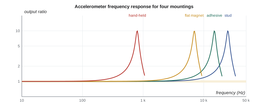
For the mechanical run test, Gilles mounts VT-401 and VT-402 on studs screwed into spot-faced pads on the TP-80's bearing housings, in the horizontal and vertical directions, as the customer's specification and the pump vibration standards ask. For quick surveys of pumps in the field, magnets are used, and the survey's report states the mounting so that readings above a kilohertz or two are treated with suspicion. The accelerometer's cable is clamped close to the sensor, because a cable that whips around generates charge of its own in some designs, and kept away from motor cables. A sensor's mass also matters on light structures: an accelerometer of 100 grams on a thin cover plate changes the plate's own vibration.
Worked problem
Choosing a speed measurement for an affinity-law correction
Test readings are corrected to rated speed by the affinity laws, with power scaling as \((n_{\text{rated}}/n)^3\). If speed is measured with a 0.1 s counting gate on ST-301, what uncertainty does the gate's resolution add to corrected power at 1,760 rpm? What if one revolution is timed instead?
Show solution
- Counting with a 0.1 s gate: ±10 rpm, a rectangular ±0.57 percent, standard uncertainty 0.33 percent.
- Corrected power varies as \(n^{-3}\) through the correction, so its relative standard uncertainty from speed is \(3 \times 0.33 = 0.98\) percent.
- Timing one revolution resolves 0.005 rpm, about 0.0003 percent; the effect on corrected power is negligible.
Answer: A short counting gate would add about one percent to the uncertainty of corrected power, more than every other source combined. Period timing, or a long gate, is essential when results are corrected by the affinity laws.
Common mistakes
MistakeUsing a short counting gate for precise speed.
InsteadTime the period over at least one revolution, or count over a long gate.
MistakeTaking high-frequency vibration readings with a hand-held probe.
InsteadStud-mount or adhesive-mount the accelerometer for readings above a few hundred hertz.
MistakeIgnoring runout on a shaft measured by proximity probes.
InsteadMeasure the slow-roll signal and treat it as a baseline.
MistakeStarting an incremental encoder system without homing.
InsteadIncremental encoders need a reference position after power-up.
MistakeFixing a heavy accelerometer to a light panel.
InsteadChoose a sensor much lighter than the structure, or the reading will be altered by its mass.
Summary and key terms
- Speed is measured by counting teeth or marks; period timing with a fast clock gives far finer resolution than short-gate counting.
- With 60 teeth, pulse frequency in hertz equals speed in rpm.
- LVDTs, magnetostrictive sensors and encoders measure position; quadrature gives four counts per line.
- Eddy-current probes measure shaft motion relative to the bearing, commonly at 7.87 V/mm, and are affected by runout.
- Piezoelectric accelerometers, often IEPE at 100 mV/g, measure acceleration over a wide band.
- Mounting sets an accelerometer's usable range: stud mounting is flat to several kilohertz, a hand-held probe to under 200 Hz.
- Magnetic pickup
- A coil and magnet that produce a pulse as each ferrous tooth passes.
- Frequency counting
- Measuring speed by counting pulses during a fixed gate time.
- Period measurement
- Measuring speed by timing the interval between pulses with a fast clock.
- LVDT
- A transformer with a movable core whose output voltage is proportional to displacement.
- Incremental encoder
- A sensor producing pulses as it moves, whose count gives relative position.
- Quadrature
- Two encoder signals a quarter cycle apart, giving direction and four counts per line.
- Eddy-current probe
- A non-contact sensor whose output depends on the gap to a conducting target.
- Runout
- False vibration signal from a shaft caused by surface or material variations.
- Piezoelectric accelerometer
- A seismic sensor in which a crystal loaded by a mass generates charge proportional to acceleration.
- Mounted resonance
- The natural frequency of an accelerometer together with its mounting.
Practice problems
Work each problem on paper first, then reveal the answer to check.
A 30-tooth wheel gives 875 Hz. What is the shaft speed?
Show answer
875 × 60/30 = 1,750 rpm.
How many counts per revolution does a 2,500-line encoder give with quadrature decoding?
Show answer
10,000.
In the program, what voltage swing would 25 µm peak-to-peak motion give at 7.87 V/mm?
Show answer
About 197 mV peak to peak.
An accelerometer reads 0.5 g peak at 176 Hz. What is the velocity amplitude?
Show answer
0.5 × 9.807/(2π × 176) = 4.4 mm/s peak.
Why is a hand-held probe unsuitable for measuring the TP-80's vane-pass vibration?
Show answer
Its mounted resonance near 800 Hz makes it inaccurate above about 180 Hz, and vane pass is 176 Hz with harmonics above.
Lesson quiz · 5 questions
Score 60% or more to complete this lesson.
Create a free account to save your progress, take quizzes and earn a certificate.