Laminar boundary layers

In 1904 Ludwig Prandtl presented a short paper that changed fluid mechanics. He argued that in a flow at high Reynolds number, viscosity matters only in a thin layer next to a solid surface, where the velocity must rise from zero at the wall to the free-stream value. Outside that layer the flow behaves as if it were inviscid, and potential flow describes it well. Inside, the Navier-Stokes equations can be simplified because the layer is thin. Prandtl's boundary layer resolved d'Alembert's paradox from Lesson 3 and made it possible to calculate skin friction, heat transfer and separation. This lesson develops the laminar boundary layer, where the mathematics is complete, and applies it to two problems from Jun's work term: the plate settlers in the treatment plant's new clarifier and a flat-plate experiment he is running with a university flume.

The boundary layer idea

Picture a thin flat plate aligned with a uniform stream U. At the leading edge the fluid in contact with the plate stops, by the no-slip condition, and the slowing spreads outward by viscous diffusion as the fluid moves downstream. The region of slowed fluid grows in thickness with distance x from the leading edge. The boundary-layer thickness δ is conventionally defined as the distance from the wall at which the velocity reaches 99 percent of U. Because the edge is approached gradually, δ is somewhat arbitrary, and two integral thicknesses with clear physical meanings are also used.

The displacement thickness δ* is the distance by which the wall would have to be moved outward, in an inviscid flow, to give the same flow rate as the real boundary layer. It measures how far the outer flow is pushed away from the wall. The momentum thickness θ measures the loss of momentum flux caused by the layer, and it is directly related to the drag on the plate:

The ratio \(H = \delta^*/\theta\), called the shape factor, describes the profile's fullness. For the laminar flat-plate profile H is about 2.59; for a turbulent profile it is about 1.3; near separation it rises toward 3.5 or more.

The boundary-layer equations

Inside a thin layer, velocities across the layer are small compared with those along it, and gradients across it are large compared with gradients along it. An order-of-magnitude analysis of the two-dimensional Navier-Stokes equations, with δ much smaller than x, drops the small terms and leaves Prandtl's boundary-layer equations:

The same analysis shows that the pressure does not change across the layer: \(\partial p/\partial y \approx 0\). The pressure inside the boundary layer is imposed by the outer flow, and the outer flow's speed U(x) enters through Bernoulli's equation as the term \(U\,dU/dx\). This is why potential flow and boundary-layer theory work together: potential flow gives the pressure distribution, and the boundary-layer equations, driven by that pressure, give the friction and tell whether the layer will separate. The analysis also gives the scaling \(\delta/x \sim 1/\sqrt{\text{Re}_x}\), where \(\text{Re}_x = Ux/\nu\).

The Blasius solution

For a flat plate at zero incidence, U is constant and the pressure gradient vanishes. Prandtl's student Heinrich Blasius showed in 1908 that the velocity profiles at different x are all the same shape when y is scaled by \(\sqrt{\nu x/U}\). With the similarity variable \(\eta = y\sqrt{U/(\nu x)}\) and a stream function written as \(\psi = \sqrt{\nu U x}\,f(\eta)\), the partial differential equations become one ordinary differential equation:

where \(f' = u/U\). There is no closed-form solution, but it is easily integrated numerically. The only unknown starting value is \(f''(0)\), and a shooting method adjusts it until \(f'\) approaches 1 far from the wall. Jun's program does exactly that with a fourth-order Runge-Kutta integration, then applies the result.

# Laminar boundary layer: Blasius solution by shooting, and the momentum-integral estimate
import math
def blasius_rhs(y):
    f, fp, fpp = y
    return [fp, fpp, -0.5 * f * fpp]
def integrate(fpp0, eta_max=10.0, n=2000):
    h = eta_max / n; y = [0.0, 0.0, fpp0]; out = [(0.0, y[1])]
    for i in range(n):          # fourth-order Runge-Kutta
        k1 = blasius_rhs(y)
        k2 = blasius_rhs([y[j] + h / 2 * k1[j] for j in range(3)])
        k3 = blasius_rhs([y[j] + h / 2 * k2[j] for j in range(3)])
        k4 = blasius_rhs([y[j] + h * k3[j] for j in range(3)])
        y = [y[j] + h / 6 * (k1[j] + 2 * k2[j] + 2 * k3[j] + k4[j]) for j in range(3)]
        out.append(((i + 1) * h, y[1]))
    return y, out
lo, hi = 0.1, 0.5               # shoot on f''(0) so that f'(infinity) = 1
for _ in range(50):
    mid = (lo + hi) / 2
    if integrate(mid)[0][1] > 1: hi = mid
    else: lo = mid
fpp0 = (lo + hi) / 2
_, prof = integrate(fpp0)
eta99 = next(e for e, u in prof if u >= 0.99)
print(f"Blasius: f''(0) = {fpp0:.4f}, u/U = 0.99 at eta = {eta99:.2f}")
print(f"  so delta = {eta99:.2f} x / sqrt(Re_x), c_f = {2*fpp0:.3f} / sqrt(Re_x)")

# Lamella settler plates in the clarifier: water speed along the plate and plate length
nu = 1.31e-6                    # m2/s at 10 C
U, Lp = 0.004, 1.5              # m/s, m
for x in (0.1, 0.5, 1.0, 1.5):
    Re_x = U * x / nu
    d = 4.91 * x / math.sqrt(Re_x)
    print(f"  x = {x:.1f} m: Re_x = {Re_x:,.0f}, delta = {d*1000:.0f} mm")
ReL = U * Lp / nu
print(f"Plate Reynolds number {ReL:,.0f}: laminar along the whole plate; the boundary layers of plates 50 mm apart meet within about {(0.025/4.91)**2*U/nu:.2f} m")

# Momentum-integral method with a parabolic profile u/U = 2(y/d) - (y/d)^2
# gives delta/x = sqrt(30) / sqrt(Re_x) and c_f = 0.730 / sqrt(Re_x)
print(f"Momentum integral, parabolic profile: delta/x = {math.sqrt(30):.2f}/sqrt(Re_x), c_f = {2/math.sqrt(30)*2:.3f}/sqrt(Re_x)")

# Test plate in the university flume: drag of both faces
rho = 999.7; U2, L2, b = 0.25, 0.40, 0.30
Re2 = U2 * L2 / nu
CD = 1.328 / math.sqrt(Re2)
F = CD * 0.5 * rho * U2**2 * (2 * L2 * b)
print(f"\nFlume plate: Re_L = {Re2:,.0f}, C_D = {CD:.5f}, drag on both faces {F:.3f} N")

Blasius: f''(0) = 0.3321, u/U = 0.99 at eta = 4.91
  so delta = 4.91 x / sqrt(Re_x), c_f = 0.664 / sqrt(Re_x)
  x = 0.1 m: Re_x = 305, delta = 28 mm
  x = 0.5 m: Re_x = 1,527, delta = 63 mm
  x = 1.0 m: Re_x = 3,053, delta = 89 mm
  x = 1.5 m: Re_x = 4,580, delta = 109 mm
Plate Reynolds number 4,580: laminar along the whole plate; the boundary layers of plates 50 mm apart meet within about 0.08 m
Momentum integral, parabolic profile: delta/x = 5.48/sqrt(Re_x), c_f = 0.730/sqrt(Re_x)

Flume plate: Re_L = 76,336, C_D = 0.00481, drag on both faces 0.036 N

The shooting method converges to \(f''(0) = 0.3321\), and the velocity reaches 99 percent of U at η = 4.91. These two numbers give the classic Blasius results for a laminar flat plate:

The local skin friction coefficient falls with distance because the layer thickens and the velocity gradient at the wall weakens. Integrating the wall shear over a plate of length L gives the average drag coefficient for one side:

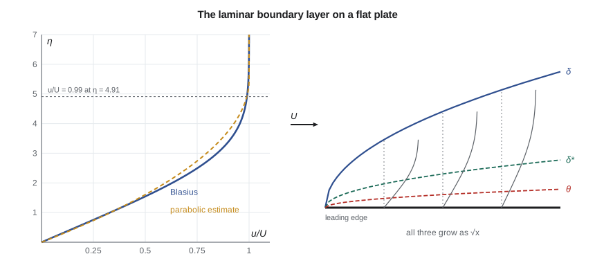
Plate settlers in the clarifier

Wascana Valley Water's new clarifier uses inclined plate settlers, also called lamella plates: stacks of parallel plates about 50 mm apart, 1.5 m long, through which water rises slowly while floc settles onto the plates and slides down. The water speed along the plates is only about 4 mm/s, and at 10 °C the kinematic viscosity is 1.31 × 10⁻⁶ m²/s. The plate Reynolds number is therefore only about 4,600, far below transition, and the flow is laminar everywhere.

The program shows that a Blasius boundary layer on an isolated plate would be 28 mm thick only 0.1 m from the leading edge and about 110 mm thick at the end. Long before that, the boundary layers on facing plates meet: with a 50 mm gap they merge about 0.08 m in, and from there on the flow between the plates is fully developed laminar channel flow, the plane Poiseuille flow of Lesson 1. This matters to the process designer, because the settling performance of plate settlers is usually analysed by assuming a parabolic velocity profile between plates. The boundary-layer calculation confirms that the entrance region, where the profile is still developing, is only a small part of the plate length.

The momentum-integral method

Before computers, the Blasius equation was integrated by hand, and engineers needed a faster method for boundary layers with pressure gradients. Theodore von Kármán supplied it in 1921 by integrating the boundary-layer momentum equation across the layer. For a flat plate the result is remarkably simple:

The wall shear equals the rate at which the momentum thickness grows. To use it, one assumes a reasonable shape for the velocity profile, expresses θ and \(\tau_w\) in terms of δ, and solves the resulting ordinary differential equation for δ(x). With a parabolic profile \(u/U = 2(y/\delta) - (y/\delta)^2\), the method gives \(\delta/x = 5.48/\sqrt{\text{Re}_x}\) and \(c_f = 0.730/\sqrt{\text{Re}_x}\), within about 10 percent of Blasius. A cubic profile does better still. The method's real value is that it extends to pressure gradients and to turbulent layers with empirical profiles, and it remains the basis of quick engineering calculations.

The flume plate experiment

Jun is helping a university research group calibrate a drag balance in a recirculating flume. A smooth plate 0.40 m long and 0.30 m wide is held edge-on in water flowing at 0.25 m/s. The plate Reynolds number is about 76,000, comfortably laminar if the leading edge is sharp and the flow is quiet. The Blasius drag coefficient is 0.0048, and the predicted drag on both faces is only 0.036 N, the weight of about 3.7 grams. The tiny force explains why laminar drag measurements need careful balances and why the measured value is often higher than Blasius: any free-stream turbulence, a rounded leading edge or vibration can trigger transition early, and a turbulent layer has several times the friction.

Pressure gradients and separation

With a favourable pressure gradient, where the outer flow accelerates and the pressure falls downstream, the boundary layer is thin and stable. In an adverse gradient, where the outer flow decelerates, the pressure rises downstream and pushes back on the slow fluid near the wall. The fluid farthest from the wall still has momentum to keep going, but the fluid near the wall has little, and eventually the wall shear falls to zero: the profile has a vertical tangent at the wall. Beyond that point the near-wall fluid flows backward and the boundary layer lifts off the surface. This is separation. Laminar layers separate easily, after only a modest pressure rise; on a circular cylinder in laminar flow they separate at about 80° from the front, before the widest point. Lesson 5 shows that turbulent layers resist separation much better, which leads to the drag crisis of Lesson 6.

Where laminar boundary layers matter

Laminar boundary layers are common at small scales and low speeds: in plate settlers, instrument probes, micro-channels, the first few centimetres of a leading edge, and the slow flows of viscous liquids. Their low friction is exploited in the design of laminar-flow airfoils and gliders, whose shapes keep the pressure falling over as much of the surface as possible to delay transition. They also matter in heat and mass transfer: the thin laminar layer at the surface of a filter grain or a membrane controls how fast dissolved substances reach it, which is why MEC-340's convection correlations had the same \(\text{Re}^{1/2}\) dependence. Most large engineering flows, however, are turbulent over most of their surfaces, and Lesson 5 takes that next step.

The clarifier's plate settlers were sized by the process engineer using the surface loading rates in the province's design standards for waterworks, which follow the widely used Great Lakes-Upper Mississippi River Board recommended standards, known as the Ten States Standards, in many details. The fluid mechanics in this lesson explains why those loading limits work: they keep the flow between plates laminar and slow.