Turbines, fans and system matching: the capstone

Jun's work term ends with a report to Hana that pulls the course together. It has four parts, each built on the turbomachinery of Lesson 11 and the external flows of Lessons 6 and 7. First, choose the type of machine for the energy-recovery turbine at the pressure-reducing station that MEC-270 sized at about 80 kW. Second, check the supply fan for the filter gallery, which runs at full speed around the clock. Third, review the developer's energy estimate for the plant's proposed wind turbine. Fourth, and most important, make the case for buying the new Pump 2 with a variable-frequency drive rather than controlling it with a throttling valve, as the old pump was. This lesson works through each part.

Turbines

A hydraulic turbine reverses the pump's role: water gives up energy to the runner, and Euler's equation, with the swirl decreasing through the runner, gives the work per unit weight. Turbines are divided into two families. In an impulse turbine, the whole head is converted into velocity in a nozzle before the water reaches the runner, which operates at atmospheric pressure. The Pelton wheel, with buckets that split and reverse a free jet, is the classic example and suits high heads, from about 100 m to well over 1,000 m. In a reaction turbine, the runner is completely filled with water and part of the pressure drop occurs in the runner itself. Francis turbines, with water entering radially and leaving axially, cover medium heads; Kaplan and propeller turbines, with axial flow through adjustable or fixed blades, cover low heads and large flows.

As with pumps, specific speed indicates the right type. For turbines it is usually written with power instead of flow, \(N_{sp} = n\sqrt{P}/H^{5/4}\), with P in kilowatts and H in metres. Pelton wheels have low values, Francis turbines intermediate ones and Kaplan turbines high ones. Turbines also cavitate, at the low-pressure exit of a reaction runner, so their setting relative to the tailwater is chosen with the Thoma number of Lesson 11, and a draft tube, a diffuser of the kind in Lesson 5, recovers the kinetic energy of the water leaving the runner.

The energy-recovery turbine at the PRV station

The pressure-reducing station on the transmission main drops the pressure from about 690 kPa to 280 kPa before the water enters a lower-pressure zone. MEC-270 found that a turbine in place of the valve could extract about 42 m of head from 0.25 m³/s, producing roughly 80 kW. The program below confirms 82 kW at 80 percent efficiency and a power specific speed of about 150 at 1,780 rpm, well inside the Francis range.

# Turbines, fans and system matching: the capstone checks
import math
g, rho = 9.81, 998.0
# 1. Energy-recovery turbine at the pressure-reducing station (MEC-270): choose the machine type
Qt, Ht, n_t = 0.25, 41.9, 1780
P_t = 0.80 * rho * g * Qt * Ht
Ns_power = n_t * math.sqrt(P_t / 1000) / Ht**1.25            # rpm, kW, m
Nq = n_t * math.sqrt(Qt) / Ht**0.75
print(f"PRV turbine: {P_t/1000:.0f} kW; power specific speed {Ns_power:.0f} (rpm, kW, m), N_q {Nq:.0f}")
for name, lo, hi in (("Pelton (impulse)", 4, 30), ("Francis", 50, 350), ("Kaplan or propeller", 350, 1000)):
    print(f"  {name:<20} roughly {lo}-{hi}", "<- this site" if lo <= Ns_power <= hi else "")
# A pump running as a turbine (PAT): common conversion factors from best-efficiency pump data
Qp, Hp = 0.21, 33.0                                          # candidate pump BEP at 1780 rpm
eta_p = 0.82
Qturb, Hturb = Qp / eta_p**0.8, Hp / eta_p**1.2              # one published estimate (a Sharma-type correlation)
print(f"Pump BEP {Qp} m3/s at {Hp} m -> as a turbine about {Qturb:.3f} m3/s at {Hturb:.1f} m")

# 2. Filter-gallery supply fan: fan laws and system matching
Q0, p0 = 6.0, 480.0                                          # fan rating point: m3/s and Pa at 1,180 rpm
fan = lambda Q, s: s**2 * 720.0 - 6.67 * Q**2                # fitted fan curve, Pa
ks = 480.0 / 36.0                                            # system: dp = ks Q^2 (no static lift)
for s in (1.0, 0.8, 0.6):
    Qop = math.sqrt(s**2 * 720.0 / (6.67 + ks))
    P = Qop * ks * Qop**2 / 0.70
    print(f"  fan at {s:.0%} speed: {Qop:.2f} m3/s, {ks*Qop**2:.0f} Pa, shaft power {P/1000:.2f} kW")

# 3. Wind turbine: Betz limit and annual energy from a Rayleigh wind distribution
p, T = 95.4e3, 273.15 + 5.0
rho_a = p / (287.0 * T)
R = 15.0; A = math.pi * R**2
a_vals = [0.1, 0.2, 1/3, 0.4, 0.5]
for a in a_vals:
    print(f"  induction a = {a:.3f}: Cp = {4*a*(1-a)**2:.3f}")
Vbar, rated = 6.0, 250e3
def power(V):
    if V < 3.5 or V > 25: return 0.0
    return min(rated, 0.5 * rho_a * A * V**3 * 0.42)        # Cp of a good modern rotor, capped at rated
E = 0.0; dV = 0.1
V = dV / 2
while V < 30:
    pdf = math.pi * V / (2 * Vbar**2) * math.exp(-math.pi / 4 * (V / Vbar) ** 2)
    E += power(V) * pdf * dV * 8760
    V += dV
print(f"Air density {rho_a:.3f} kg/m3; annual energy {E/1e6:.0f} MWh, capacity factor {E/(rated*8760):.0%}")

# 4. Capstone: replacement Pump 2 with a variable-frequency drive against throttling
H0, a, dz, ksys = 78.0, 210.0, 48.0, 63.9
eta = lambda Q: 0.86 * (1 - ((Q - 0.32) / 0.32) ** 2)       # full-speed efficiency curve
duty = ((0.33, 2500), (0.28, 3200), (0.24, 2200))            # flow (m3/s) and hours per year
E_thr = E_vfd = 0.0
for Qd, hrs in duty:
    Hthr = H0 - a * Qd**2                                    # throttled: stay on the full-speed curve
    P_thr = rho * g * Qd * Hthr / eta(Qd) / 0.95
    s = math.sqrt((dz + ksys * Qd**2 + a * Qd**2) / H0)      # speed that meets the system curve at Qd
    Qeq = Qd / s                                             # equivalent full-speed flow (affinity)
    Hv = dz + ksys * Qd**2
    P_vfd = rho * g * Qd * Hv / eta(Qeq) / (0.95 * 0.97)     # motor and drive losses
    E_thr += P_thr * hrs / 1e6; E_vfd += P_vfd * hrs / 1e6
    print(f"  {Qd:.2f} m3/s: throttled {Hthr:.1f} m, {P_thr/1000:.0f} kW; VFD {s:.0%} speed, {Hv:.1f} m, {P_vfd/1000:.0f} kW")
print(f"Annual energy: throttling {E_thr:.0f} MWh, VFD {E_vfd:.0f} MWh, saving {E_thr-E_vfd:.0f} MWh")

PRV turbine: 82 kW; power specific speed 151 (rpm, kW, m), N_q 54
  Pelton (impulse)     roughly 4-30 
  Francis              roughly 50-350 <- this site
  Kaplan or propeller  roughly 350-1000 
Pump BEP 0.21 m3/s at 33.0 m -> as a turbine about 0.246 m3/s at 41.9 m
  fan at 100% speed: 6.00 m3/s, 480 Pa, shaft power 4.11 kW
  fan at 80% speed: 4.80 m3/s, 307 Pa, shaft power 2.11 kW
  fan at 60% speed: 3.60 m3/s, 173 Pa, shaft power 0.89 kW
  induction a = 0.100: Cp = 0.324
  induction a = 0.200: Cp = 0.512
  induction a = 0.333: Cp = 0.593
  induction a = 0.400: Cp = 0.576
  induction a = 0.500: Cp = 0.500
Air density 1.195 kg/m3; annual energy 546 MWh, capacity factor 25%
  0.33 m3/s: throttled 55.1 m, 218 kW; VFD 100% speed, 55.0 m, 224 kW
  0.28 m3/s: throttled 61.5 m, 210 kW; VFD 94% speed, 53.0 m, 184 kW
  0.24 m3/s: throttled 65.9 m, 202 kW; VFD 90% speed, 51.7 m, 158 kW
Annual energy: throttling 1662 MWh, VFD 1498 MWh, saving 164 MWh

A purpose-built Francis turbine of 80 kW is an expensive, custom machine. For small sites like this one, utilities often use a standard centrifugal pump run in reverse as a turbine, abbreviated PAT. It costs a fraction as much, is available quickly and can be serviced like the utility's other pumps; its peak efficiency is a few points lower than a custom turbine's and it has no adjustable guide vanes, so it works best at a steady flow. A pump running as a turbine needs a higher head and flow than its pump rating to reach its best efficiency. One published estimate, often credited to Sharma, scales the turbine flow by the pump efficiency to the −0.8 power and the head by the efficiency to the −1.2 power. The program shows that a standard pump rated at 0.21 m³/s and 33 m, with 82 percent efficiency, should reach its best efficiency as a turbine at about 0.25 m³/s and 42 m, a good match for the station. The estimate is approximate; the supplier's test data for the pump in turbine mode is needed before purchase.

Fans and the fan laws

Fans are turbomachines for gases at pressure rises small enough that the gas can be treated as incompressible, typically below about 7 to 10 kPa. Above that, blowers and compressors take over and the compressible relations of Lessons 8 to 10 apply. Centrifugal fans with backward-inclined or airfoil blades are efficient and have stable, non-overloading power curves, like pumps with backward-curved blades. Forward-curved fans are compact and quiet but less efficient. Axial fans move large volumes at low pressure. The fan laws are the affinity laws in another form: flow proportional to speed, pressure to speed squared and power to speed cubed, with a correction for air density when it differs from the rating condition.

The filter gallery's supply fan delivers 6.0 m³/s against 480 Pa at full speed. A ventilation duct system has no static lift, so its resistance is proportional to the square of the flow, and the system curve passes through the origin. On such a system, the operating point follows the fan laws exactly, which the program confirms: at 80 percent speed the fan delivers 80 percent of the flow at 64 percent of the pressure, and its shaft power falls from 4.1 kW to 2.1 kW. At night, when the gallery is unoccupied, 60 percent speed would meet the minimum ventilation rate for 0.9 kW. The saving of more than 3 kW for 12 hours a day is about 14 MWh a year, which pays for a drive on a fan this size in a year or two.

The wind turbine and the Betz limit

A wind turbine extracts kinetic energy from the air passing through its rotor. A simple momentum analysis, due to Rankine, Froude and Betz, treats the rotor as an actuator disk that slows the wind from V far upstream to V(1 − a) at the disk and V(1 − 2a) far downstream. Applying mass, momentum and energy conservation to the stream tube through the disk gives the power and power coefficient:

No rotor can extract more than 59.3 percent of the kinetic energy flowing through its area. Slowing the wind too much backs the air up and diverts it around the rotor; slowing it too little leaves energy in the wake. Real rotors lose more to blade drag, wake swirl and tip losses, and the best modern rotors reach power coefficients of about 0.45 to 0.5 at their design tip-speed ratio. The blade-section aerodynamics of Lesson 7 determines how close a design comes to the limit.

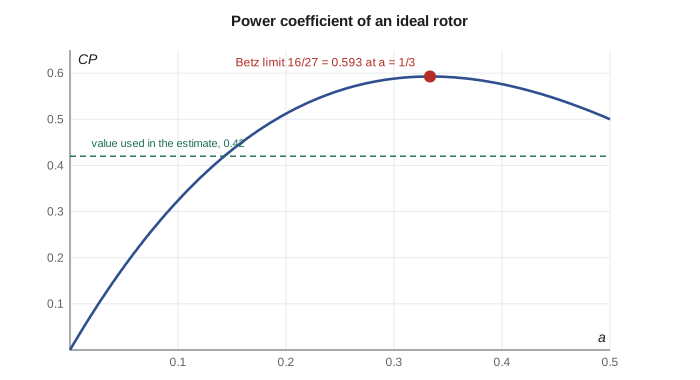
Because wind speed varies, a turbine's annual energy depends on the distribution of wind speeds at its hub, not just the mean. A Rayleigh distribution, a Weibull distribution with shape factor 2, is a common first estimate when only the mean speed is known. The program combines it with a simplified power curve: zero below a cut-in speed of 3.5 m/s, \(\tfrac12\rho A V^3\) times an overall power coefficient of 0.42 up to the rated power of 250 kW, and zero above a cut-out speed of 25 m/s. With the developer's hub-height mean of 6.0 m/s and the local air density, the estimate is about 546 MWh a year, a capacity factor of about 25 percent. Because power varies with the cube of wind speed, a 10 percent error in the mean wind changes the energy by roughly 20 to 30 percent, which is why Hana insists on at least a year of measured data from a met mast at hub height before the board commits.

The air at Regina, about 580 m above sea level, is about 6 percent less dense than at sea level, which lowers the energy by the same fraction. The developer's estimate used sea-level density; correcting it is one of Jun's review comments. In Canada, wind resource assessments for projects of this size commonly use the national wind atlas as a screening tool before site measurements.

System matching: Pump 2 with a variable-frequency drive

The heart of Jun's report is the control method for Pump 2. Northside's demand varies with the season and the time of day. The old pump ran at full speed and a throttling valve on its discharge reduced the flow when less was needed, which adds an artificial head loss and moves the operating point up the pump curve. A variable-frequency drive instead lowers the pump's speed, moving the curve down until it meets the system curve at the required flow, as in Lesson 11. The program compares the two methods over a year with three duty points: 0.33 m³/s for 2,500 hours, 0.28 m³/s for 3,200 hours and 0.24 m³/s for 2,200 hours. For the drive, it applies the affinity laws to find the efficiency at each reduced speed and includes 3 percent drive losses.

At full flow the drive is slightly worse than a direct-on-line motor, 224 kW against 218 kW, because of its own losses. At the lower flows it is much better. At 0.28 m³/s the throttled pump must still generate 61.5 m, of which only 53 m is needed; the drive runs the pump at 94 percent speed and saves 26 kW. At 0.24 m³/s it saves 44 kW. Over the year, the drive uses about 1,500 MWh instead of 1,660 MWh, a saving of about 164 MWh, or roughly 18,000 dollars a year at 0.11 dollars per kWh. Against an extra cost of about 60,000 dollars for a drive of this size, the payback is between three and four years.

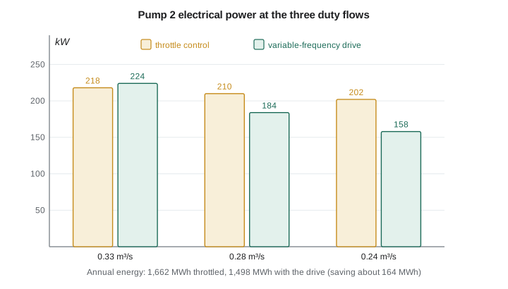
The savings are smaller than the cube law would suggest, because the 48 m static lift does not shrink with speed. That is the general lesson of system matching: the benefit of speed control depends on the ratio of friction head to static head. In circulating systems, such as chilled-water loops, district energy networks and the filter-gallery fan, where friction dominates, savings are large. In lifting systems with high static head, such as Northside, they are moderate, and the drive also brings other benefits: soft starting that reduces water hammer, the ability to hold a constant reservoir level, and protection against running the pump at shutoff.

Jun's recommendations

Jun's report to Hana sums up the term. For the PRV station, a pump running as a turbine of about 80 kW, with a bypass valve for pressure control, earning about 490 MWh a year. For the filter gallery, a variable-frequency drive on the supply fan, with night setback to 60 percent speed. For the wind turbine, a year of hub-height wind measurements before any decision, and an energy estimate corrected for local air density. For Pump 2, the Tidewater pump as designed, with a variable-frequency drive, a minimum speed of 85 percent, and a 0.5 m higher minimum clearwell level to protect the NPSH margin in summer. Each recommendation rests on fluid mechanics learned in this course: dimensional analysis and similitude, potential flow and boundary layers, drag and lift, compressible flow and the theory of turbomachines.

Capital projects for Canadian utilities of this kind are normally reviewed by a professional engineer before approval, and energy-saving projects may qualify for incentive programs offered by the provincial electric utility. Hana will seal the final design of the PRV turbine and Pump 2 installation, and the utility's application to the province will include Jun's energy calculations.