Differential analysis and the Navier-Stokes equations

Jun Park is back at Wascana Valley Water for his second work term, this time in the capital projects group. In Fluid Mechanics I he checked the Northside pumping station with control volumes: a box drawn around a bend, a pump or a whole pipeline, with mass, momentum and energy balanced across its faces. That approach gave him forces on anchors and the head a pump must deliver without knowing anything about what happens inside the box. This term his projects need more. Hana Lindqvist, the utility's senior engineer, has handed him a list: a new raw-water intake on the Qu'Appelle River, a replacement for Pump 2, an air-valve review on the transmission main, a wind turbine proposal for the treatment plant and a wind check on the elevated reservoir. Each needs the distribution of velocity or pressure, not just totals: the shear on a surface, the drag of a body, the flow pattern near an intake, the speed of air through a valve. That calls for differential analysis, where the conservation laws are applied to an infinitesimal element and solved for the whole flow field.

This lesson derives the differential forms of mass and momentum conservation for a Newtonian fluid, which are the Navier-Stokes equations, and solves them exactly for a handful of simple flows that occur all over a water utility: flow in a small dosing tube, the oil film in a pump bearing and a thin film running down a ramp. Those exact solutions are the foundation for boundary layers in Lessons 4 and 5, and the limits of their validity are a first look at turbulence.

From control volumes to a field description

A control-volume balance answers questions about inflow and outflow. A differential balance answers questions about every point. The trade is effort: instead of one algebraic equation, the engineer faces partial differential equations for the velocity components u, v and w and the pressure p as functions of position and time. In return the solution gives everything, including the wall shear stress that sets friction, the pressure distribution that sets drag and lift, and the places where the flow may separate.

The element is a small rectangular box of sides dx, dy and dz fixed in space. Mass enters and leaves through its six faces, and forces act on its faces through pressure and viscous stress. Writing the balances and letting the box shrink to a point gives equations valid everywhere in the flow. MEC-270 introduced the material derivative, the rate of change following a fluid particle, which appears in every term that involves acceleration:

The first term is the local acceleration, present only in unsteady flow. The other three are convective acceleration, which exists even in steady flow whenever a particle moves into a region of different velocity, as it does in a nozzle or around a bend. Convective acceleration is nonlinear, because the velocity multiplies its own gradient, and that nonlinearity is the main reason fluid mechanics is hard.

Conservation of mass in differential form

The net rate at which mass flows out of the element must equal the rate at which the mass inside it decreases. For the x faces, the mass flow in is \(\rho u\,dy\,dz\) and the flow out is that value plus its change across the box. Adding the three directions and dividing by the volume gives the continuity equation:

For an incompressible fluid, where density is constant, it reduces to a statement that the velocity field has zero divergence:

This simple equation is surprisingly powerful. In a two-dimensional flow, it shows that if u decreases along a wall, v must increase away from it: fluid slowed by friction near a surface is pushed outward. It also lets the velocity field be described by a single stream function, used in Lesson 3. Water at the pressures in a distribution system is incompressible for this purpose; its density changes by less than 0.05 percent per megapascal. Air in a low-speed fan duct can also be treated as incompressible, but air in a valve, a nozzle or a blower discharge at high speed cannot, which is the subject of Lessons 8 to 10.

Stresses in a moving fluid

At rest, a fluid supports only pressure, which acts equally in all directions. In motion it also carries viscous stresses that resist deformation. For a Newtonian fluid, such as water, air and light oils, the viscous stresses are proportional to the rates of strain. In two dimensions the stresses on the element are:

The shear stress \(\tau_{xy}\) is the generalization of Newton's law of viscosity \(\tau = \mu\,du/dy\) from MEC-270. The normal stresses include both pressure and a viscous part that acts when the fluid is stretched or squeezed. Non-Newtonian fluids, such as the thick sludge from the plant's clarifiers or concentrated polymer, do not follow these relations: their apparent viscosity depends on the shear rate, and their pipe flow needs other models. The dilute polymer solution used in this lesson is close enough to Newtonian at its working concentration for the exact solution to be useful.

The Navier-Stokes equations

Newton's second law for the element sets its mass times acceleration equal to the body force plus the net surface force. Substituting the Newtonian stresses and the incompressible continuity equation gives, in vector form:

and in the x direction, written out:

Each term has a physical meaning. The left side is inertia, the mass per unit volume times acceleration. On the right, the pressure gradient pushes fluid from high to low pressure, gravity acts on the mass, and the viscous term diffuses momentum from fast-moving to slow-moving fluid. Together with continuity, the three momentum equations give four equations for four unknowns, u, v, w and p. They were derived in the first half of the nineteenth century by Navier and Stokes, among others, and they describe essentially every flow an engineer meets, from the polymer feed line to the wind around the water tower.

Two special cases are worth naming. When viscosity is negligible, the viscous term drops out and the result is Euler's equation, whose integral along a streamline is the Bernoulli equation of MEC-270. When inertia is negligible, as in very slow flow of a viscous fluid or flow of very small particles, the left side drops out and the result is the Stokes or creeping flow equation, used in Lesson 6 for settling grit. The ratio of inertia to viscous forces is the Reynolds number, and Lesson 2 shows how it emerges when the equations are written in dimensionless form.

Boundary conditions

Equations alone do not define a flow; the boundaries do. At a solid wall a viscous fluid obeys the no-slip condition: the fluid in contact with the wall moves with the wall. It also cannot pass through an impermeable wall. At an inlet or outlet the velocity or pressure is specified. At a free surface, such as the water in the intake channel, the pressure equals atmospheric pressure and the shear stress is nearly zero. The no-slip condition is what produces shear stress, friction drag and boundary layers; without it, flows past bodies would have no drag at all, a famous paradox discussed in Lesson 3.

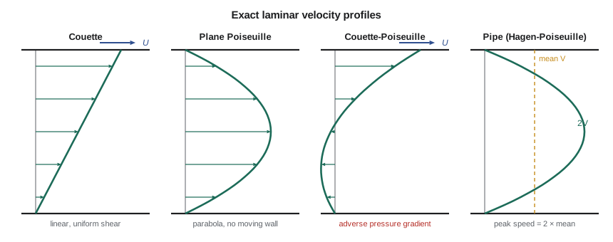
Exact solution 1: Couette flow

Consider fluid between two very wide parallel plates a distance h apart. The lower plate is fixed and the upper plate moves at speed U, with no pressure gradient along the flow. If the flow is steady and fully developed, so that u depends only on y and v = w = 0, continuity is satisfied automatically and every inertia term vanishes. The x momentum equation reduces to:

after applying u = 0 at y = 0 and u = U at y = h. The velocity varies linearly, and the shear stress \(\tau = \mu U/h\) is the same everywhere in the gap. This is the model for a lubricated journal bearing when the film is thin compared with the shaft radius and the shaft is centred. MEC-360 used the same result, Petroff's equation, for the TM-4 multistage pump. Here it gives the friction in the oil-lubricated guide bearing of a vertical turbine pump that Wascana Valley Water uses at its raw-water intake.

Exact solution 2: Poiseuille flow in a pipe

In a long, straight round pipe, laminar flow far from the inlet is fully developed: the velocity is axial and depends only on the radius r. In cylindrical coordinates the axial momentum equation reduces to a balance between the pressure gradient and viscous shear:

Integrating twice, requiring a finite velocity on the centreline and no slip at the wall r = R, gives the parabolic Hagen-Poiseuille profile, the flow rate and the pressure drop:

The friction factor that follows, \(f = 64/\text{Re}\), was used in MEC-270 without proof; it is one of the few results in fluid mechanics that comes straight from the governing equations with no empirical constants. The strong dependence on diameter is the practical lesson: halving a laminar line's diameter raises its pressure drop sixteenfold at the same flow.

Wascana Valley Water feeds a dilute polymer flocculant aid from a day tank to the flash mixer through a 20 mm tube 38 m long. The flow is 150 L/h, and the solution has a viscosity of about 0.045 Pa·s, roughly 45 times that of water. Ray Mendoza, the senior operator, wants to know whether the metering pump can deliver it and what the tube's pressure drop will be when the solution is made up stronger in winter. The program below solves this case along with the bearing and a falling film.

# Exact laminar solutions of the Navier-Stokes equations applied at Wascana Valley Water
import math
g = 9.81

# 1. Poiseuille flow: polymer feed line from the day tank to the flash mixer
mu, rho = 0.045, 1005.0           # Pa.s and kg/m3 for the dilute polymer solution (treated as Newtonian)
D, L = 0.020, 38.0                # tube diameter and length, m
Q = 150 / 1000 / 3600             # 150 L/h in m3/s
V = Q / (math.pi * D**2 / 4)
Re = rho * V * D / mu
dp = 128 * mu * L * Q / (math.pi * D**4)
tau_w = 4 * mu * (2 * V) / D       # wall shear = mu du/dr at the wall, u_max = 2V
print(f"Polymer line: V = {V:.3f} m/s, Re = {Re:.1f} (laminar), pressure drop = {dp/1000:.2f} kPa")
print(f"  centreline speed {2*V:.3f} m/s, wall shear stress {tau_w:.3f} Pa")
for r_frac in (0.0, 0.25, 0.5, 0.75, 1.0):
    u = 2 * V * (1 - r_frac**2)
    print(f"  r/R = {r_frac:.2f}: u = {u:.3f} m/s")

# 2. Couette flow: oil film in the guide bearing of a vertical turbine pump
mu_oil = 0.030                    # Pa.s at running temperature
Dj, Lj, c = 0.080, 0.100, 0.10e-3 # journal diameter, length and radial clearance, m
n = 1780                          # rpm
U = math.pi * Dj * n / 60
tau = mu_oil * U / c              # linear profile: shear stress is uniform across the film
F = tau * math.pi * Dj * Lj
T = F * Dj / 2
P = T * 2 * math.pi * n / 60
print(f"\nGuide bearing: surface speed {U:.2f} m/s, shear stress {tau/1000:.1f} kPa")
print(f"  friction torque {T:.2f} N.m, power lost {P:.0f} W")

# 3. Falling film on the cascade aerator ramp: laminar film solution and a reality check
nu = 1.0e-6                       # m2/s, water near 20 C
theta = math.radians(30)
for q in (1e-5, 1e-4, 0.05):      # flow per metre of width, m2/s
    h = (3 * nu * q / (g * math.sin(theta))) ** (1 / 3)
    Re_f = q / nu
    print(f"film flow q = {q:g} m2/s: laminar thickness {h*1000:.3f} mm, Re = {Re_f:,.0f}",
          "(laminar solution valid)" if Re_f < 500 else "(turbulent: the exact solution does not apply)")

Polymer line: V = 0.133 m/s, Re = 59.2 (laminar), pressure drop = 18.14 kPa
  centreline speed 0.265 m/s, wall shear stress 2.387 Pa
  r/R = 0.00: u = 0.265 m/s
  r/R = 0.25: u = 0.249 m/s
  r/R = 0.50: u = 0.199 m/s
  r/R = 0.75: u = 0.116 m/s
  r/R = 1.00: u = 0.000 m/s

Guide bearing: surface speed 7.46 m/s, shear stress 2.2 kPa
  friction torque 2.25 N.m, power lost 419 W
film flow q = 1e-05 m2/s: laminar thickness 0.183 mm, Re = 10 (laminar solution valid)
film flow q = 0.0001 m2/s: laminar thickness 0.394 mm, Re = 100 (laminar solution valid)
film flow q = 0.05 m2/s: laminar thickness 3.127 mm, Re = 50,000 (turbulent: the exact solution does not apply)

The polymer line runs at a Reynolds number of about 59, deep in the laminar range, so the exact solution applies with confidence. The pressure drop of about 18 kPa is well within the metering pump's capacity. If the operators double the concentration and the viscosity triples, the pressure drop triples too, because the laminar drop is proportional to viscosity; at 55 kPa the pump still copes, but the tube fittings and the pump's relief setting should be checked.

Exact solution 3: a film flowing down a ramp

The treatment plant's cascade aerator spreads raw water in a thin sheet down a series of inclined steps to strip dissolved gases. A sheet of liquid flowing steadily down a wide plane inclined at angle θ, with a free surface on top, is another exact solution. Gravity's component along the plane drives the flow, the wall imposes no slip and the free surface has zero shear. The profile is a half-parabola, and the film thickness for a flow q per unit width is:

The program shows that the result is valid for trickle flows but not for the aerator's design flow. At 0.05 m² of flow per second per metre of width the film Reynolds number is about 50,000: the sheet is turbulent and wavy, and the laminar solution would give a film only 3 mm thick when the real sheet is several times thicker. This is the first and most important lesson about exact solutions: they are exact only while the flow stays laminar. Most engineering flows of water and air are turbulent, and for them the Navier-Stokes equations remain true but no longer have simple solutions.

Combined Couette-Poiseuille flow

When a moving wall and a pressure gradient act together, the two solutions add, because the reduced equation is linear. Between a fixed plate and a plate moving at U, with pressure gradient dp/dx:

If the pressure rises in the direction of motion, an adverse gradient, the second term is negative and can overcome the first near the fixed wall, producing backflow. This is a simplified picture of the slider bearing that carries the thrust in large vertical pumps, where the converging wedge builds pressure, and it is also a first view of what happens in a boundary layer facing an adverse pressure gradient: the slow fluid near the wall reverses and the flow separates. Lesson 5 returns to separation.

Vorticity and irrotational flow

The differential view also gives a precise way to describe rotation. The vorticity vector \(\boldsymbol{\omega} = \nabla \times \mathbf{V}\) measures twice the local angular velocity of fluid particles. In Couette flow the vorticity is \(-U/h\) everywhere: particles in a shear flow rotate even though every streamline is straight. Viscosity creates vorticity at walls and diffuses it into the flow. Far from walls, in flows that started from rest or from a uniform stream, the vorticity is often negligible. Such flows are called irrotational. For them the Navier-Stokes equations collapse to the much simpler Laplace equation for a velocity potential, the subject of Lesson 3, and Bernoulli's equation applies between any two points, not just along a streamline.

Computational fluid dynamics

Only a few dozen exact solutions of the Navier-Stokes equations are known, and almost all of them are laminar. For real geometries, engineers solve the equations numerically. Computational fluid dynamics divides the flow into millions of cells and solves discretized forms of continuity and momentum in each. For turbulent flows the equations are usually averaged in time, which introduces extra stresses that must be modelled with turbulence models such as k-ε or k-ω SST. The results depend on mesh quality, the turbulence model and the boundary conditions, so CFD is checked against exact solutions, experiments and the kind of hand calculations in this course. Tidewater Pump Works, the Moncton pump maker that will supply the new Pump 2, uses CFD to shape impellers and a physical model test, the subject of Lesson 2, to confirm the result.

Engineers in Canada who seal CFD-based designs are responsible for checking them like any other calculation. Provincial regulators such as the Association of Professional Engineers and Geoscientists of Saskatchewan expect the engineer to understand and verify software results, and exact solutions like those in this lesson are the standard way to confirm that a model reproduces known behaviour.