Laplace transforms · MATH-201 Lesson 4

Real engineering inputs are rarely smooth sine waves. A switch closes, a valve slams shut, a hammer strikes, a load is suddenly applied. The methods of Lesson 2 struggle with inputs like these. The Laplace transform handles them gracefully: it turns a linear differential equation into an algebraic equation, builds in the initial conditions automatically, and treats switching and impulses as easily as smooth functions.

It also gives engineers a new way of thinking about systems. The transfer function, a ratio of polynomials in a variable s, captures everything about how a linear system responds, and it is the foundation of control engineering, signal processing and circuit analysis. This chapter defines the transform, builds a working table, solves initial value problems with it, handles step and impulse inputs, and introduces transfer functions.

The definition

The Laplace transform of a function $f(t)$, defined for $t \ge 0$, is

\[\mathcal{L}\{f(t)\} = F(s) = \int_0^\infty e^{-st} f(t)\,dt\]

It turns a function of time into a function of a new variable s (which can be complex; for now think of it as a real number large enough for the integral to converge). Capital letters denote transforms: $Y(s) = \mathcal{L}\{y(t)\}$.

Worked problem

Transform of an exponential

Find $\mathcal{L}\{e^{at}\}$.

Show solution

\[\int_0^\infty e^{-st}e^{at}\,dt = \int_0^\infty e^{-(s - a)t}\,dt = \left[\frac{-e^{-(s-a)t}}{s - a}\right]_0^\infty = \frac{1}{s - a}\]
This converges for $s > a$. With $a = 0$, $\mathcal{L}\{1\} = 1/s$.

Answer: 1/(s − a). For example, e^{t} has transform 1/(s − 1), and at s = 3 the integral ∫₀^∞ e^{−3t}e^{t} dt = 1/2, as a numerical check confirms

Nobody evaluates these integrals routinely. Engineers work from a table, built once from the definition.

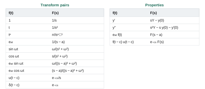
A table of Laplace transform pairs: 1 to 1 over s; t to 1 over s squared; t to the n to n factorial over s to the n plus 1; e to the at to 1 over s minus a; sin omega t to omega over s squared plus omega squared; cos omega t to s over s squared plus omega squared; e to the at times sin omega t to omega over (s minus a) squared plus omega squared; e to the at cos omega t to (s minus a) over (s minus a) squared plus omega squared; unit step u(t minus c) to e to the minus cs over s; impulse delta(t minus c) to e to the minus cs. Below, properties: derivative y prime transforms to sY minus y(0); y double prime to s squared Y minus s y(0) minus y prime(0); shifting e to the at f(t) to F(s minus a). — A working table of transforms and properties. With these, most engineering IVPs can be solved.

Two properties make the transform useful.

Linearity: $\mathcal{L}\{af + bg\} = aF + bG$.
Derivatives become multiplication by s, with the initial conditions appearing automatically:

\[\mathcal{L}\{y'\} = sY - y(0), \qquad \mathcal{L}\{y''\} = s^2Y - s\,y(0) - y'(0)\]

The derivative rule follows from integrating the definition by parts. It is the reason the method works: differentiation in time becomes algebra in s.

Solving initial value problems

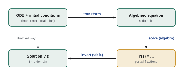
The method has three steps: transform the equation, solve the algebraic equation for $Y(s)$, and invert to get $y(t)$, usually by splitting $Y(s)$ into partial fractions that appear in the table.

$A flow diagram. Top left: ODE plus initial conditions in the time domain. Arrow labelled transform goes right to an algebraic equation in s. Arrow down labelled solve for Y(s). Arrow left labelled inverse transform with partial fractions, back to the solution y(t) in the time domain. A dashed arrow straight down on the left labelled hard way connects the ODE to the solution.$

The Laplace transform method: a detour through the s-domain replaces calculus with algebra.

Worked problem

A first-order problem

Solve $y' + 2y = 4$, $y(0) = 0$.

Show solution

Transform: $sY - 0 + 2Y = 4/s$, so $Y = \dfrac{4}{s(s + 2)}$.
Partial fractions: $\dfrac{4}{s(s + 2)} = \dfrac{A}{s} + \dfrac{B}{s + 2}$. Cover-up: $A = 4/2 = 2$ (set s = 0 in the rest), $B = 4/(-2) = -2$ (set s = −2).
Invert: $y = 2 - 2e^{-2t}$.

Answer: y = 2(1 − e^{−2t}), the same as Lesson 1 found with an integrating factor

Worked problem

A second-order problem

Solve $y'' + 3y' + 2y = 0$, $y(0) = 1$, $y'(0) = 0$.

Show solution

Transform: $(s^2Y - s) + 3(sY - 1) + 2Y = 0$, so $(s^2 + 3s + 2)Y = s + 3$.
$Y = \dfrac{s + 3}{(s + 1)(s + 2)} = \dfrac{2}{s + 1} - \dfrac{1}{s + 2}$ (cover-up: at s = −1, $2/1 = 2$; at s = −2, $1/(-1) = -1$).
Invert: $y = 2e^{-t} - e^{-2t}$.

Answer: y = 2e^{−t} − e^{−2t}. The denominator s² + 3s + 2 is exactly the characteristic polynomial: its roots (the poles of Y) give the exponents of the response

Worked problem

Complex roots by completing the square

Solve $y'' + 2y' + 5y = 0$, $y(0) = 1$, $y'(0) = 0$ by Laplace transform.

Show solution

Transform: $(s^2 + 2s + 5)Y = s + 2$, so $Y = \dfrac{s + 2}{s^2 + 2s + 5}$.
Complete the square: $s^2 + 2s + 5 = (s + 1)^2 + 4$. Write the numerator as $(s + 1) + 1$:
\[Y = \frac{s + 1}{(s + 1)^2 + 2^2} + \frac{1}{2}\cdot\frac{2}{(s + 1)^2 + 2^2}\]
From the table (shifted cosine and sine): $y = e^{-t}\cos 2t + \tfrac{1}{2}e^{-t}\sin 2t$.

Answer: y = e^{−t}(cos 2t + ½ sin 2t), matching Lesson 2. Complex poles −1 ± 2i signal a decaying oscillation

Switching: the unit step

The unit step (Heaviside) function switches from 0 to 1 at time c:

\[u(t - c) = \begin{cases} 0 & t < c \\ 1 & t \ge c \end{cases}, \qquad \mathcal{L}\{u(t - c)\} = \frac{e^{-cs}}{s}\]

A delayed function is handled by the second shifting theorem: $\mathcal{L}\{f(t - c)\,u(t - c)\} = e^{-cs}F(s)$. In words: a factor $e^{-cs}$ in the s-domain means "the same response, delayed by c".

Worked problem

Switching on a circuit late

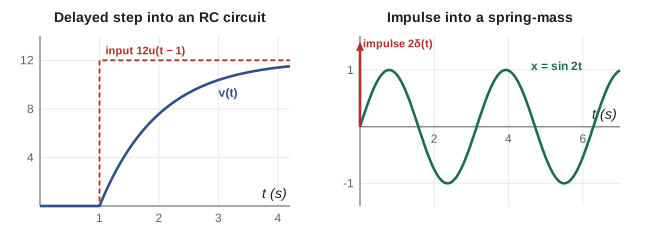
An RC circuit with $\tau = 1$ s starts uncharged. A 12 V source is switched on at $t = 1$ s. Find v(t).

Show solution

Equation: $v' + v = 12\,u(t - 1)$, $v(0) = 0$.
Transform: $(s + 1)V = 12e^{-s}/s$, so $V = 12e^{-s}\cdot\dfrac{1}{s(s + 1)}$.
$\dfrac{1}{s(s + 1)} = \dfrac{1}{s} - \dfrac{1}{s + 1}$, whose inverse is $1 - e^{-t}$.
The factor $e^{-s}$ delays it by 1 s: $v = 12\left(1 - e^{-(t - 1)}\right)u(t - 1)$.

Answer: Zero until t = 1 s, then the familiar charging curve starting at t = 1. At t = 3 s, v = 12(1 − e⁻²) = 10.4 V, which a numerical solution confirms

Left: the delayed step input switching from 0 to 12 V at t = 1 s and the capacitor voltage, zero until 1 s and then rising toward 12 V. Right: an impulse at t = 0 drawn as a tall spike, and the response of an undamped spring-mass system, a sine wave starting at zero. — A delayed step input to an RC circuit (left) and an impulse applied to a spring-mass system (right).

Impulses

A hammer blow, a collision or a lightning strike delivers a large force for a very short time. Its effect depends on the impulse (force × time, from PHYS-130), not on the details of its shape. The idealization is the Dirac delta $\delta(t - c)$: zero except at $t = c$, with total area 1. Its transform is remarkably simple:

\[\mathcal{L}\{\delta(t - c)\} = e^{-cs}, \qquad \mathcal{L}\{\delta(t)\} = 1\]

Worked problem

A hammer test

A 1 kg mass on a spring with k = 4 N/m (no damping) is at rest. At t = 0 it is struck with an impulse of 2 N·s. Find its motion.

Show solution

Equation: $x'' + 4x = 2\delta(t)$, $x(0) = x'(0) = 0$.
Transform: $(s^2 + 4)X = 2$, so $X = \dfrac{2}{s^2 + 4}$.
From the table, $\mathcal{L}\{\sin 2t\} = 2/(s^2 + 4)$, so $x = \sin 2t$.

Answer: x = sin 2t (metres): it starts at zero with velocity 2 m/s (impulse ÷ mass) and oscillates at the natural frequency, 2 rad/s. Impact (hammer) tests on real structures use exactly this idea to excite and measure their natural frequencies

Transfer functions

For a linear system starting at rest, transforming the equation gives $Y(s) = G(s)\,F(s)$: output equals transfer function times input. For the mass-spring-damper, $m\ddot{x} + c\dot{x} + kx = f(t)$ gives

\[G(s) = \frac{X(s)}{F(s)} = \frac{1}{ms^2 + cs + k}\]

The transfer function depends only on the system, not on the input. Its poles (roots of the denominator) are the characteristic roots, and they determine stability and the natural response. Engineers describe and connect systems by their transfer functions, multiplying them for components in series. Control engineering is largely the art of designing a controller transfer function that moves the poles of the overall system to good places.

Two handy results follow. The impulse response is the inverse transform of G itself (since $F = 1$). And the final value theorem gives the steady state without inverting anything: if the response settles,

\[\lim_{t \to \infty} y(t) = \lim_{s \to 0} s\,Y(s)\]

Worked problem

Steady deflection under a suddenly applied load

A suddenly applied constant force $F_0$ (a step) acts on the quarter-car model (m = 300 kg, c = 1800 N·s/m, k = 30 kN/m). Find the final deflection using the final value theorem, and the system's poles.

Show solution

$X(s) = G(s)\,\dfrac{F_0}{s}$. Final value: $\lim_{s\to 0} s \cdot \dfrac{1}{ms^2 + cs + k}\cdot\dfrac{F_0}{s} = \dfrac{F_0}{k}$.
Poles: $300s^2 + 1800s + 30\,000 = 0$, or $s^2 + 6s + 100 = 0$: $s = -3 \pm 9.54i$.

Answer: Final deflection F₀/k, the static value, as it must be. The poles −3 ± 9.54i show a decaying oscillation at 9.54 rad/s, settling with time constant 1/3 s, matching ζ = 0.3 and ωn = 10 from Lesson 3

Convolution, briefly

If the input is an arbitrary function, $Y = GF$ in the s-domain corresponds in time to the convolution $y(t) = \int_0^t g(\tau)f(t - \tau)\,d\tau$, where g is the impulse response. Physically, the response is the sum of the responses to all the little impulses that make up the input. This is the basis of how earthquake engineers compute a building's response to a recorded ground motion, and how audio software applies the acoustics of a concert hall to a recording.

Common mistakes

MistakeForgetting the initial-condition terms in L{y′} and L{y″}.
InsteadL{y′} = sY − y(0); L{y″} = s²Y − s y(0) − y′(0).
MistakeInverting without partial fractions, guessing from the whole expression.
InsteadSplit Y(s) into table forms first; check by recombining.
MistakeIgnoring the delay factor e^{−cs} when inverting.
InsteadInvert the rest, then shift by c and multiply by u(t − c).
MistakeLeaving complex quadratic denominators unfactored and stuck.
InsteadComplete the square to (s − a)² + ω² and use the shifted sine and cosine pairs.
MistakeApplying the final value theorem to an unstable or oscillating system.
InsteadIt is valid only if y(t) actually settles; check that all poles of sY(s) have negative real parts.
MistakeMixing up the transform of sin (ω on top) and cos (s on top).
InsteadL{sin ωt} = ω/(s² + ω²); L{cos ωt} = s/(s² + ω²).

Summary and key terms

L{f} = ∫₀^∞ e^{−st} f(t) dt turns functions of t into functions of s; use a table rather than the integral.
Linearity, and L{y′} = sY − y(0), L{y″} = s²Y − s y(0) − y′(0), turn linear ODEs into algebra with initial conditions built in.
Method: transform, solve for Y(s), split into partial fractions, invert from the table.
Poles of Y(s) are the characteristic roots and determine the form of the response.
Steps u(t − c) transform to e^{−cs}/s; a factor e^{−cs} delays a response by c.
An impulse δ(t) transforms to 1, so the impulse response is the inverse of the transfer function.
Transfer function G(s) = output/input for a system at rest; final value lim y = lim_{s→0} sY(s) when the response settles.

Laplace transform: F(s) = ∫₀^∞ e^{−st} f(t) dt.
Inverse transform: Recovering f(t) from F(s), usually from a table after partial fractions.
Partial fractions: Splitting a rational function into simpler terms that appear in the table.
Pole: A value of s where a transform's denominator is zero.
Unit step function: u(t − c), which switches from 0 to 1 at t = c.
Dirac delta: δ(t), an idealized impulse of unit area at t = 0.
Transfer function: G(s), the ratio of output to input transforms for a system starting at rest.
Impulse response: A system's response to δ(t); the inverse transform of G(s).
Final value theorem: lim_{t→∞} y(t) = lim_{s→0} sY(s), when the limit exists.
Convolution: The time-domain operation corresponding to multiplying transforms.

Practice problems

Work each problem on paper first, then reveal the answer to check.

Find L{3 − 2t + e^{−4t}}.
Show answer
3/s − 2/s² + 1/(s + 4).
Find L{e^{−2t} cos 3t}.
Show answer
(s + 2)/((s + 2)² + 9).
Find the inverse transform of 5/(s(s + 5)).
Show answer
1/s − 1/(s + 5) → 1 − e^{−5t}.
Find the inverse transform of (2s + 1)/(s² + 4).
Show answer
2 cos 2t + ½ sin 2t.
Solve y′ − 3y = 0, y(0) = 4, by Laplace transform.
Show answer
sY − 4 − 3Y = 0, Y = 4/(s − 3), y = 4e^{3t}.
Solve y″ + 4y′ + 3y = 0, y(0) = 0, y′(0) = 2.
Show answer
(s² + 4s + 3)Y = 2, Y = 2/((s + 1)(s + 3)) = 1/(s + 1) − 1/(s + 3). y = e^{−t} − e^{−3t}.
Solve y″ + y = 1, y(0) = y′(0) = 0.
Show answer
Y = 1/(s(s² + 1)) = 1/s − s/(s² + 1). y = 1 − cos t.
Find L{u(t − 2)(t − 2)}.
Show answer
e^{−2s}/s².
For G(s) = 5/(s² + 2s + 5) and a unit step input, find the final value of the output.
Show answer
lim_{s→0} s · G(s) · (1/s) = 5/5 = 1.
What are the poles of G(s) = 1/(s² + 0.4s + 4), and what do they say about the response?
Show answer
s = −0.2 ± 1.99i: a lightly damped oscillation at about 2 rad/s (ζ = 0.1), stable.