Eigenvalues and eigenvectors

When a matrix multiplies a vector, the vector usually changes direction. But almost every square matrix has a few special directions that it leaves alone, stretching or shrinking vectors along them without turning them. Those directions are the eigenvectors, and the stretch factors are the eigenvalues.

This may sound like a curiosity, but eigenvalues are among the most useful ideas in engineering. The natural frequencies at which a bridge, a building or a turbine blade vibrates are eigenvalues. The principal stresses that decide whether a part yields are eigenvalues. Whether a control system or a chemical reactor is stable depends on eigenvalues, and so does the long-run behaviour of any process that repeats step after step. This chapter shows how to find them, what they mean and how they are used.

The idea

A non-zero vector \(\mathbf{v}\) is an eigenvector of the square matrix \(A\) if multiplying by \(A\) only scales it:

The scale factor \(\lambda\) (lambda) is the eigenvalue belonging to \(\mathbf{v}\). If \(\lambda = 3\), vectors in that direction are stretched to three times their length. If \(\lambda = 0.5\) they are halved; if \(\lambda\) is negative they are flipped; if \(\lambda = 0\) they are crushed to zero. The zero vector is excluded, since \(A\mathbf{0} = \lambda\mathbf{0}\) for every \(\lambda\) and would tell us nothing.

Any multiple of an eigenvector is also an eigenvector with the same eigenvalue, because \(A(c\mathbf{v}) = cA\mathbf{v} = \lambda(c\mathbf{v})\). So an eigenvector really names a direction, a whole line through the origin. You can scale it however is convenient.

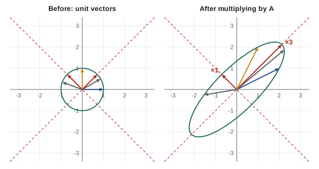
The picture shows something more. The eigenvectors point along the axes of the ellipse that the unit circle becomes. In the eigenvector directions, the matrix is just a pair of independent stretches. That is the main reason eigenvectors are useful: they are the natural coordinates in which a complicated matrix becomes simple.

Finding eigenvalues: the characteristic equation

Rewrite \(A\mathbf{v} = \lambda\mathbf{v}\) as \(A\mathbf{v} - \lambda I\mathbf{v} = \mathbf{0}\), that is:

This homogeneous system has a non-zero solution \(\mathbf{v}\) only if \(A - \lambda I\) is singular (Lesson 4). So the eigenvalues are exactly the numbers that make its determinant zero:

This is the characteristic equation. For an \(n \times n\) matrix, the determinant is a polynomial of degree \(n\) in \(\lambda\), so there are \(n\) eigenvalues counting repeats, though some may be complex.

The procedure:

• Subtract \(\lambda\) from each diagonal entry and set the determinant equal to zero.
• Solve the polynomial for the eigenvalues.
• For each eigenvalue, solve \((A - \lambda I)\mathbf{v} = \mathbf{0}\) by elimination. There will always be at least one free variable (that is what singular means). Choose a convenient value for it.

Two quick checks

For any square matrix, the eigenvalues add up to the trace (the sum of the diagonal entries) and multiply to the determinant:

For the last example: \(5 + 2 = 7 = 4 + 3\) and \(5 \times 2 = 10 = 12 - 2\). For 2×2 matrices this means the characteristic equation is always \(\lambda^2 - (\operatorname{tr} A)\lambda + \det A = 0\), which is the fastest way to write it down. It also shows that a matrix is singular exactly when 0 is one of its eigenvalues.

A 3×3 example

For larger matrices the characteristic polynomial is harder to factor, so look for structure, such as a row or column with zeros.

Beyond 3×3, nobody finds eigenvalues by factoring polynomials. Software uses iterative methods (the QR algorithm, or the power method below) that never form the polynomial at all.

Special cases

Symmetric matrices

Symmetric matrices, which include stiffness matrices, stress tensors and inertia tensors, are the best-behaved case. Their eigenvalues are always real, and eigenvectors belonging to different eigenvalues are always perpendicular. A symmetric \(n \times n\) matrix always has \(n\) perpendicular eigenvector directions. Engineering relies on this guarantee every day.

Complex eigenvalues

A rotation turns every vector, so in the real plane it has no eigenvector directions at all. The algebra agrees: for the 90° rotation \(\begin{pmatrix} 0 & -1 \\ 1 & 0 \end{pmatrix}\), the characteristic equation is \(\lambda^2 + 1 = 0\), so \(\lambda = \pm i\). Complex eigenvalues signal rotation or oscillation. In a dynamic system they mean the response oscillates, and their real part says whether the oscillation grows or decays. You will rely on this in differential equations and control courses.

Repeated eigenvalues

The shear \(\begin{pmatrix} 1 & 1 \\ 0 & 1 \end{pmatrix}\) has characteristic equation \((1 - \lambda)^2 = 0\), so \(\lambda = 1\) twice. But \(A - I = \begin{pmatrix} 0 & 1 \\ 0 & 0 \end{pmatrix}\) gives only \(y = 0\), so there is only one eigenvector direction, \((1, 0)\). A matrix like this, with fewer independent eigenvectors than its size, is called defective. Symmetric matrices are never defective.

Diagonalization and matrix powers

Suppose an \(n \times n\) matrix has \(n\) independent eigenvectors. Put them as the columns of a matrix \(P\), and put the eigenvalues on the diagonal of \(D\). The equations \(A\mathbf{v}_i = \lambda_i\mathbf{v}_i\) together say \(AP = PD\), so

This is diagonalization. It says that in eigenvector coordinates, \(A\) acts like the diagonal matrix \(D\): an independent stretch along each axis. Its first big payoff is powers. Because the inner \(P^{-1}P\) pairs cancel,

and powers of a diagonal matrix just raise each diagonal entry to the power.

The long-run behaviour is now obvious: the largest eigenvalue dominates. As \(k\) grows, \(3^k\) swamps \(1^k\), and \(A^k\mathbf{x}\) lines up with the eigenvector \((1, 1)\) for almost any starting \(\mathbf{x}\). If every eigenvalue had absolute value less than 1, \(A^k\mathbf{x}\) would die away to zero; if any exceeds 1, it grows. That is the stability test for any process that repeats a linear step.

The power method

The same observation gives a simple way to compute the dominant eigenvalue numerically: start with almost any vector and keep multiplying by \(A\). Starting from \((1, 0)\) with the matrix above gives \((2, 1)\), \((5, 4)\), \((14, 13)\), \((41, 40)\), \((122, 121)\). The direction approaches \((1, 1)\), and the ratio of successive lengths approaches 3 (for instance \(122/41 \approx 2.98\)). Search engines have used variants of this method on matrices with billions of rows.

Engineering applications

Principal stresses

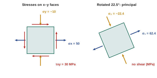
The state of stress at a point in a loaded part is described by a symmetric stress matrix. In two dimensions it is \(\begin{pmatrix} \sigma_x & \tau_{xy} \\ \tau_{xy} & \sigma_y \end{pmatrix}\), with normal stresses on the diagonal and shear stress off it. Rotating the axes changes these numbers. In the eigenvector directions the shear vanishes, and the normal stresses there, the eigenvalues, are the largest and smallest normal stresses at that point. These principal stresses are what failure criteria for metals and concrete are written in terms of.

Mechanics of materials teaches the same result through Mohr's circle, a graphical way of finding these eigenvalues.

Natural frequencies and mode shapes

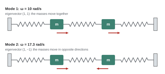
A structure vibrating freely obeys \(M\ddot{\mathbf{x}} = -K\mathbf{x}\), where \(M\) is the mass matrix and \(K\) the stiffness matrix. Looking for motions in which every part oscillates at the same frequency, \(\mathbf{x} = \mathbf{v}\cos\omega t\), turns this into an eigenvalue problem: \(K\mathbf{v} = \omega^2 M\mathbf{v}\). The eigenvalues give the natural frequencies and the eigenvectors give the mode shapes, the pattern in which the structure moves.

If a machine or the wind drives a structure near one of its natural frequencies, the response can grow very large: resonance. Engineers compute these eigenvalues for every building in an earthquake zone, every aircraft wing and every rotating shaft, and design to keep them away from the frequencies of the expected loads.

Long-run behaviour of a repeated process