
MATH-125 · Lesson 12 of 12 · 28 min
Linear algebra in engineering: case studies and a project
Linear algebra is the computational backbone of modern engineering. Structural analysis, circuit simulation, control design, signal processing, computer graphics, machine learning and the finite element method all reduce, at their core, to vectors, matrices, linear systems and eigenvalue problems. This course has built the tools: vectors and their combinations (Lessons 1 and 2), linear systems and their efficient solution (Lessons 3 and 5), matrix algebra and determinants (Lessons 4 and 6), the structure of solutions (Lesson 7), transformations (Lesson 8), eigenvalues (Lessons 9 and 11), and least squares (Lesson 10). This final lesson applies them together in three case studies, each typical of a different engineering discipline, and then sets a course project. The emphasis is on formulating problems in matrix form, which is the step that software cannot do for you, and on interpreting the results.
Case study 1: forces in a truss
A truss carries loads through members that are in pure tension or compression. Its analysis is a linear system: at each joint, the member forces and external loads must balance in both directions. Consider a triangular truss with joints A at (0, 0), B at (4, 0) and C at (2, 2) metres, members AB, AC and BC, a pin support at A (reactions \(A_x\), \(A_y\)), a roller at B (reaction \(B_y\)), and a 10 kN downward load at C. Member forces \(F_{AB}\), \(F_{AC}\), \(F_{BC}\) are taken positive in tension.
- Each member force acts along the member, so it contributes its force times a unit vector to each joint it connects. The unit vector from C toward A is \((-1, -1)/\sqrt{2}\), from C toward B is \((1, -1)/\sqrt{2}\), and from A toward B is \((1, 0)\).
- Three joints give six equations in six unknowns (three member forces and three reactions), so the system is square, matching the count of Lesson 7 for a determinate truss.
Worked problem
Solving the truss
Write the equilibrium equations and solve for the member forces and reactions.
Show solution
- Joint C: \(\tfrac{1}{\sqrt{2}}(-F_{AC} + F_{BC}) = 0\) and \(\tfrac{1}{\sqrt{2}}(-F_{AC} - F_{BC}) - 10 = 0\). So \(F_{AC} = F_{BC} = -7.07\) kN.
- Joint B: \(-F_{AB} - \tfrac{1}{\sqrt{2}}F_{BC} = 0\), so \(F_{AB} = 5\) kN; and \(\tfrac{1}{\sqrt{2}}F_{BC} + B_y = 0\), so \(B_y = 5\) kN.
- Joint A: \(F_{AB} + \tfrac{1}{\sqrt{2}}F_{AC} + A_x = 0\), so \(A_x = 0\); \(\tfrac{1}{\sqrt{2}}F_{AC} + A_y = 0\), so \(A_y = 5\) kN.
Answer: The inclined members carry 7.07 kN in compression, the bottom chord 5 kN in tension, and each support 5 kN upward. Here the equations could be solved one joint at a time, but in a large truss the 2j × (m + r) equilibrium matrix is assembled and solved by LU factorization (Lesson 5), and its rank (Lesson 7) checks that the truss is stable.
In the stiffness method used by structural software, the unknowns are the joint displacements instead of the forces. Each member contributes a small symmetric stiffness matrix, and these are assembled into a global stiffness matrix \(K\), which is symmetric, sparse and, for a properly supported structure, positive definite. The structure's response to loads \(\mathbf{f}\) is found by solving \(K\mathbf{u} = \mathbf{f}\), usually by Cholesky factorization, and its natural vibrations from the eigenvalue problem \(K\boldsymbol{\phi} = \omega^2M\boldsymbol{\phi}\) of Lesson 11. The finite element method extends the same assembly process to plates, shells and solids with millions of unknowns.
Case study 2: nodal analysis of a circuit
Circuit simulators write Kirchhoff's current law at each node in terms of the unknown node voltages, giving a linear system \(G\mathbf{v} = \mathbf{i}\), where \(G\) is the conductance matrix and \(\mathbf{i}\) holds the source currents injected at each node. Each conductance \(1/R\) connecting two nodes adds to both their diagonal entries and subtracts from the two corresponding off-diagonal entries, so \(G\) is symmetric; a conductance to ground adds only to the diagonal.
Worked problem
A two-node circuit
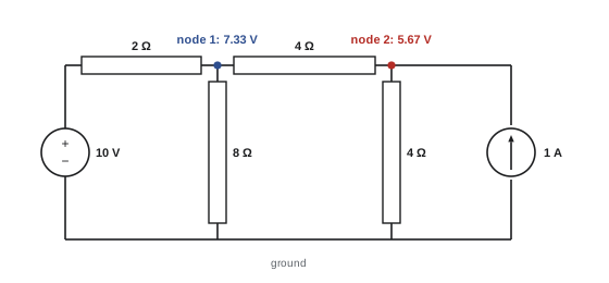
Node 1 connects to a 10 V source through 2 Ω, to node 2 through 4 Ω, and to ground through 8 Ω. Node 2 connects to ground through 4 Ω and receives a 1 A source current. Find the node voltages.
Show solution
- Replace the 10 V source and 2 Ω resistor by an equivalent current source of \(10/2 = 5\) A into node 1 in parallel with 2 Ω.
- Conductance matrix: \(G = \begin{pmatrix} \tfrac{1}{2} + \tfrac{1}{4} + \tfrac{1}{8} & -\tfrac{1}{4} \\ -\tfrac{1}{4} & \tfrac{1}{4} + \tfrac{1}{4} \end{pmatrix} = \begin{pmatrix} 0.875 & -0.25 \\ -0.25 & 0.5 \end{pmatrix}\); \(\mathbf{i} = (5, 1)\).
- From the second equation, \(v_2 = 2 + 0.5v_1\); substituting, \(0.875v_1 - 0.5 - 0.125v_1 = 5\), so \(v_1 = 7.33\) V and \(v_2 = 5.67\) V.
Answer: v₁ = 7.33 V and v₂ = 5.67 V. The conductance matrix is symmetric and diagonally dominant, hence positive definite, so the system always has a unique solution and Cholesky factorization or Gauss-Seidel iteration (Lesson 5) works well. Power system engineers solve the same kind of system, with complex admittances (MATH-101, Lesson 9), for networks of thousands of buses.
Case study 3: reliability as a Markov chain
Many systems move randomly between a few states: a machine may be running, degraded or failed; a traffic signal's queue may be short, medium or long; a customer may be with one supplier or another. A Markov chain models such a system with a transition matrix \(P\) whose entry \(p_{ij}\) is the probability of moving from state \(j\) to state \(i\) in one time step. Each column sums to 1. If \(\mathbf{x}_k\) holds the probabilities of being in each state at step \(k\), then \(\mathbf{x}_{k+1} = P\mathbf{x}_k\), and \(\mathbf{x}_k = P^k\mathbf{x}_0\), a matrix power of the kind computed with eigenvalues in Lesson 9.
A transition matrix always has the eigenvalue 1, and for most practical chains its eigenvector, scaled so its entries sum to 1, is the steady-state distribution that the system approaches regardless of where it starts. The other eigenvalues, all smaller than 1 in magnitude, determine how quickly the approach happens.
Worked problem
Long-run availability of a pump
Each week, a running pump stays running with probability 0.90, becomes degraded with probability 0.08 and fails with probability 0.02. A degraded pump is restored to running by maintenance with probability 0.3, stays degraded with probability 0.6 and fails with probability 0.1. A failed pump is repaired with probability 0.5 and otherwise stays failed. Find the long-run fraction of weeks in each state.
Show solution
- \[P = \begin{pmatrix} 0.90 & 0.30 & 0.50 \\ 0.08 & 0.60 & 0 \\ 0.02 & 0.10 & 0.50 \end{pmatrix}\]
- Solve \((P - I)\boldsymbol{\pi} = \mathbf{0}\) with \(\pi_1 + \pi_2 + \pi_3 = 1\). The second row gives \(0.08\pi_1 = 0.4\pi_2\), so \(\pi_2 = 0.2\pi_1\); the third gives \(0.02\pi_1 + 0.1\pi_2 = 0.5\pi_3\), so \(\pi_3 = 0.08\pi_1\).
- Normalize: \(\pi_1(1 + 0.2 + 0.08) = 1\), so \(\pi_1 = 0.781\), \(\pi_2 = 0.156\), \(\pi_3 = 0.0625\).
Answer: In the long run the pump runs 78 percent of the time, is degraded 16 percent and failed 6 percent. The other eigenvalues have magnitude about 0.51, so the system forgets its starting state within a few weeks. Changing the maintenance probability and recomputing the eigenvector shows how much availability a better maintenance programme buys, the kind of analysis that supports reliability-centred maintenance (DCE-450).
What the case studies share
In each case study, the engineering content lay in setting up the matrix: choosing unknowns, writing one equation per balance law (forces at a joint, currents at a node, probabilities into a state), and recognizing the structure of the resulting matrix. Once set up, the computations used standard tools whose properties this course has explained: symmetric positive definite systems solved reliably by factorization, ranks that confirm a model is well posed, and eigenvectors that describe long-run or natural behaviour. Recognizing these structures tells an engineer which software method to choose and what could go wrong.
Linear algebra and computation
In practice, engineers carry out these calculations with numerical software: MATLAB, Python with the NumPy and SciPy libraries, Julia, spreadsheets for small problems, and specialized programs for structures, circuits and fluids. All of them call the same core numerical libraries, developed over decades, that implement the LU, Cholesky, QR, eigenvalue and singular value algorithms described in this course. Using them well requires understanding what they compute: that solving is better than inverting, that symmetric positive definite matrices deserve a Cholesky solver, that a warning about a near-singular matrix signals a modelling problem, and that the condition number limits the accuracy of any answer. ENCM-100 introduces programming for these computations.
The course project
Choose one of the following problems, or propose your own of similar scope with your instructor's approval, and prepare a technical report with your formulation, calculations (by hand for small cases and with software for larger ones), results and interpretation.
- Project A: Truss analysis. Design a planar truss with at least seven members for a stated span and load. Assemble the equilibrium matrix, check its rank for stability and determinacy, solve for the member forces, and identify the most heavily loaded members. Then add one member and describe the null space of self-stresses that appears.
- Project B: Circuit or pipe network. Analyse a resistive circuit with at least four nodes, or a water distribution network linearized around an operating point, by nodal analysis. Show that the matrix is symmetric and positive definite, solve it by Cholesky or Gauss-Seidel, and check the solution against Kirchhoff's laws.
- Project C: Data fitting. Collect or obtain a data set from an engineering source (a calibration, a material test, a temperature record). Fit at least two candidate models by least squares, compare their residuals, check for overfitting by holding back some data, and discuss which model you would use and why.
- Project D: Vibration or Markov model. Model a multi-storey frame, a vehicle suspension or a chain of masses and springs, and find its natural frequencies and mode shapes; or model a system that moves between states (equipment condition, traffic, inventory) as a Markov chain, and find its steady state and how fast it is reached.
Every report should define the unknowns and assumptions, show how each equation follows from a physical law, state the size, structure and rank of the matrices, verify the solution independently, discuss sensitivity to the most uncertain inputs, and interpret the results in engineering terms.
Looking ahead
Linear algebra continues throughout an engineering program. Multivariable calculus (MATH-209) uses vectors and matrices to describe gradients, Jacobians and coordinate changes. Differential equations (MATH-201) solves systems of equations using the eigenvalues and eigenvectors of Lesson 9, and numerical methods (MATH-300) develops the algorithms of Lessons 5 and 10 further. Structural analysis, the finite element method, circuit and power system analysis, control systems, robotics and machine learning all build directly on this course.
Common mistakes
MistakeWriting equilibrium equations without a consistent sign convention for member forces.
InsteadTake tension positive and use unit vectors pointing away from each joint along each member.
MistakeAssembling a conductance matrix that is not symmetric.
InsteadEach resistor between two nodes adds to both diagonals and subtracts from both off-diagonals.
MistakeUsing a transition matrix whose columns do not sum to 1.
InsteadEach column (from-state) must hold probabilities summing to 1.
MistakeSolving a model without checking its rank or conditioning.
InsteadConfirm that the matrix is well posed before trusting the solution.
MistakeReporting numbers without interpretation.
InsteadExplain what the forces, voltages or probabilities mean for the design.
Summary and key terms
- Engineering models become linear systems by writing one balance equation per joint, node or state.
- Truss equilibrium gives a square system for a determinate truss; its rank confirms stability.
- The stiffness method assembles a sparse symmetric positive definite matrix solved by Cholesky.
- Nodal analysis gives a symmetric, diagonally dominant conductance matrix.
- Markov chains evolve by x_(k+1) = Px_k; the steady state is the eigenvector for eigenvalue 1.
- Software implements LU, Cholesky, QR, eigenvalue and SVD algorithms; understanding them guides their use.
- The course project applies formulation, computation, verification and interpretation to an engineering system.
- Truss
- A structure of pin-connected members carrying axial forces.
- Equilibrium matrix
- The matrix relating member forces and reactions to joint loads.
- Stiffness method
- Structural analysis in terms of joint displacements and a stiffness matrix.
- Global stiffness matrix
- The assembled matrix K relating displacements to loads.
- Nodal analysis
- Circuit analysis using node voltages as unknowns.
- Conductance matrix
- The matrix G relating node voltages to injected currents.
- Markov chain
- A random process whose next state depends only on the current state.
- Transition matrix
- The matrix of state-to-state probabilities.
- Steady-state distribution
- The long-run probabilities of a Markov chain.
- Availability
- The long-run fraction of time a system is operational.
Practice problems
Work each problem on paper first, then reveal the answer to check.
A truss has 4 joints, 5 members and 3 reactions. How many equations and unknowns?
Show answer
8 equations, 8 unknowns.
In the triangle truss, what force would the inclined members carry under a 20 kN load?
Show answer
14.1 kN in compression.
Why is a global stiffness matrix positive definite for a supported structure?
Show answer
Every non-zero displacement stores positive strain energy.
Write G for two nodes joined by 5 Ω, each connected to ground by 10 Ω.
Show answer
[[0.3, −0.2], [−0.2, 0.3]].
Solve that circuit with 1 A injected into node 1 only.
Show answer
v₁ = 6 V, v₂ = 4 V.
What must each column of a transition matrix sum to?
Show answer
1.
A two-state chain has P = [[0.9, 0.4], [0.1, 0.6]]. Steady state?
Show answer
(0.8, 0.2).
Starting in state 1, what is x₁ for that chain?
Show answer
(0.9, 0.1).
What determines how fast a Markov chain approaches steady state?
Show answer
The magnitude of its second-largest eigenvalue.
Name three numerical factorizations implemented by engineering software.
Show answer
LU, Cholesky, QR (also eigenvalue and SVD algorithms).
Lesson quiz · 5 questions
Score 60% or more to complete this lesson.
Create a free account to save your progress, take quizzes and earn a certificate.