Voltage regulation and reactive power from inverters

Leo's hosting-capacity screen in lesson 7 treated the feeder as if it started at exactly nominal voltage. Marguerite sends him back to the SCADA records: \"Look at what Lincoln Road's bus actually does at light load, then run a real power flow.\" This lesson builds that power flow, adds Birch Hill to it in several reactive power modes, and looks at how the utility's own voltage regulating equipment, designed for one-way flow, behaves when a large resource sits on the feeder.

How distribution voltage is regulated

Distribution utilities keep customer voltage within limits with a small set of devices. At the substation, an on-load tap changer (LTC) on the power transformer, or a separate bus regulator, raises or lowers the bus voltage in steps of about 0.625 %. Its controller often uses line-drop compensation (LDC): it estimates the voltage drop along the feeder from the current it measures and raises the bus voltage as load grows, so that the voltage at a chosen point down the feeder stays roughly constant. Along long feeders, step-voltage regulators boost the voltage again. Switched capacitor banks supply reactive power, reducing the current and the voltage drop during heavy load.

Every one of those devices was designed assuming that power flows from the substation toward the load and that voltage falls with distance. A large generator on the feeder breaks both assumptions. It reduces or reverses the current that the LTC's line-drop compensation measures, so the LTC may lower the bus voltage just when the feeder's far end needs it. It reverses power flow through line regulators, which, unless set for bidirectional or cogeneration operation, may regulate the wrong side or run their taps to the limit. And the voltage profile may now rise from the substation to the generator instead of falling.

A power flow of feeder F2

Leo models F2 as eighteen one-kilometre sections of the trunk conductor, with light-load demand of 2 MW at 0.95 power factor spread evenly along it, and the substation bus held at 1.025 pu, which is where the LTC sits on light-load days according to the SCADA history. He solves it with a backward–forward sweep, the standard method for radial feeders: starting from a guess of the voltages, he sums currents from the end of the feeder back to the substation, then steps forward from the substation computing voltage drops, and repeats until nothing changes. The inverter's reactive power, when it depends on voltage, is updated each iteration with some damping so that the solution converges smoothly, much as the inverter's own control responds over a few seconds.

import math, cmath
# Backward-forward sweep power flow on feeder F2 with Birch Hill tapped at 11 km
Sb, Vb = 10e6, 24.94e3; Zb = Vb**2/Sb                 # 10 MVA base
N, DKM = 18, 1.0                                      # 1 km sections
zsec = complex(0.11, 0.40)*DKM/Zb
VS = 1.025                                            # LTC holds the 25 kV bus at 1.025 pu at light load
def run(load_mw, mode, poi=11):
    p_load = load_mw/N/10; q_load = p_load*math.tan(math.acos(0.95))
    q_der = 0.0; v = [VS + 0j]*(N + 1)
    for it in range(60):
        s = [0j]*(N + 1)
        for k in range(1, N + 1): s[k] = -complex(p_load, q_load)          # loads (generator convention)
        if mode != 'off':
            s[poi] += complex(1.0, q_der)                                    # 10 MW = 1.0 pu
        # backward: section currents
        i = [0j]*(N + 2)
        for k in range(N, 0, -1): i[k] = i[k + 1] + (s[k]/v[k]).conjugate()
        # forward: voltages
        for k in range(1, N + 1): v[k] = v[k - 1] + i[k]*zsec
        vp = abs(v[poi])
        if mode == 'pf0.95': q_target = -math.tan(math.acos(0.95))
        elif mode == 'voltvar':                                              # IEEE 1547 Cat B default curve, Q in pu of 1.1 pu S
            pts = [(0.92, 0.44), (0.98, 0.0), (1.02, 0.0), (1.08, -0.44)]
            if vp <= pts[0][0]: qp = pts[0][1]
            elif vp >= pts[-1][0]: qp = pts[-1][1]
            else:
                for (v1, q1), (v2, q2) in zip(pts, pts[1:]):
                    if v1 <= vp <= v2: qp = q1 + (q2 - q1)*(vp - v1)/(v2 - v1)
            q_target = qp*1.1
        else: q_target = 0.0
        q_der += 0.5*(q_target - q_der)                                      # damped update
    losses = sum(abs(i[k])**2*zsec.real for k in range(1, N + 1))*10
    return [abs(x) for x in v], q_der*10, losses
for mode in ('off', 'pf1', 'pf0.95', 'voltvar'):
    v, q, loss = run(2.0, mode)
    print(f"light load, Birch Hill {mode:8s}: V at POI {v[11]:.4f} pu, max {max(v):.4f} pu, end {v[18]:.4f} pu, "
          f"Q {q:+5.2f} Mvar, feeder losses {loss*1000:4.0f} kW")
v, q, loss = run(12.0, 'voltvar')
print(f"peak load,  Birch Hill voltvar : V at POI {v[11]:.4f} pu, end {v[18]:.4f} pu, Q {q:+5.2f} Mvar")
v, q, loss = run(12.0, 'off')
print(f"peak load,  Birch Hill off     : V at POI {v[11]:.4f} pu, end {v[18]:.4f} pu")

light load, Birch Hill off     : V at POI 1.0189 pu, max 1.0250 pu, end 1.0177 pu, Q +0.00 Mvar, feeder losses    5 kW
light load, Birch Hill pf1     : V at POI 1.0360 pu, max 1.0360 pu, end 1.0348 pu, Q +0.00 Mvar, feeder losses  134 kW
light load, Birch Hill pf0.95  : V at POI 1.0129 pu, max 1.0250 pu, end 1.0117 pu, Q -3.29 Mvar, feeder losses  167 kW
light load, Birch Hill voltvar : V at POI 1.0303 pu, max 1.0303 pu, end 1.0291 pu, Q -0.83 Mvar, feeder losses  138 kW
peak load,  Birch Hill voltvar : V at POI 1.0070 pu, end 0.9997 pu, Q +0.00 Mvar
peak load,  Birch Hill off     : V at POI 0.9861 pu, end 0.9786 pu

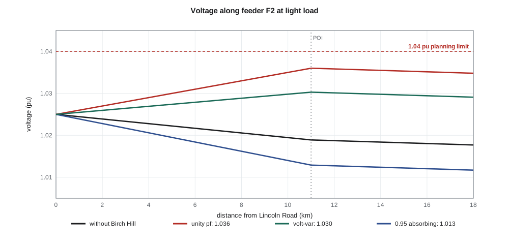
Without Birch Hill the light-load profile falls gently from 1.025 pu to about 1.018 pu at the end of the feeder. With Birch Hill exporting 10 MW at unity power factor, the voltage at the point of interconnection rises to 1.036 pu, and the whole far half of the feeder sits near that value. Larchmont's planning limit for the 25 kV primary is 1.04 pu, chosen so that customers' service voltage stays within the national range after the drop through their transformers and services. The margin is only 0.4 %, which leaves little room for higher substation voltage, measurement error or future projects.

With the plant absorbing reactive power at a fixed power factor of 0.95, the POI voltage falls to 1.013 pu, below the bus voltage. The rise is completely cancelled, but at a cost: the 3.3 Mvar the plant absorbs must flow out along the feeder from the substation, raising feeder losses from 134 kW to 167 kW at this load, and the reactive power must ultimately come from somewhere in the transmission system. At peak load, a fixed absorbing power factor would also depress voltage when the feeder needs support.

Volt-var control

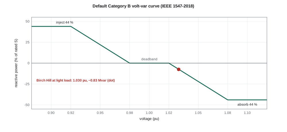
Volt-var control makes the inverter's reactive power a function of the voltage it measures. IEEE 1547-2018 specifies a default curve for Category B resources: zero reactive power in a deadband between 0.98 and 1.02 pu, rising linearly to full injection of about 44 % of rated apparent power at 0.92 pu, and to full absorption of the same amount at 1.08 pu. The utility may adjust the points within allowed ranges. Because reactive power is drawn only when voltage leaves the deadband, the plant absorbs little at ordinary voltages, supports voltage when it sags, and pulls voltage down when it rises.

In Leo's model the volt-var curve settles at 1.030 pu at the POI with the plant absorbing 0.83 Mvar, a compromise between unity power factor and fixed absorption. Losses rise only slightly, to 138 kW. At peak load the plant's voltage sits inside the deadband and it supplies no reactive power, and the POI voltage is 1.007 pu instead of 0.986 pu without the plant, because the plant's real power now offsets part of the load current. Volt-var therefore helps at both ends of the load range, which is why many utilities now make it the default mode for new inverter-based resources.

Other inverter voltage functions

Several other functions complement volt-var. Watt-var control sets reactive power as a function of the plant's real output, absorbing more when the plant exports more; it needs no voltage measurement and is predictable, but it ignores the actual voltage. Volt-watt control reduces real power when voltage exceeds a high threshold; it acts as a safety net that keeps voltage below the upper limit when reactive power alone is not enough, at the cost of lost energy. Constant reactive power and constant power factor are simple and predictable but cannot adapt to conditions. Many utilities combine modes, for example volt-var with volt-watt as a backstop.

Reactive power has another subtle cost. When an inverter is at its apparent power limit, more reactive power means less real power, so a utility that demands large reactive absorption during the sunniest hours may force the plant to curtail energy, a choice the standards call reactive priority. Birch Hill's 11 MVA of solar inverters can absorb 4.6 Mvar at 10 MW without curtailment, so with volt-var's 0.83 Mvar there is no conflict. On a plant whose inverters were rated exactly at its megawatt output, there would be.

Coordinating with the utility's own equipment

Adding Birch Hill also changes how Lincoln Road's equipment behaves. Leo's model holds the bus at 1.025 pu, but the real LTC's line-drop compensation sees the feeder's current fall, or reverse, when Birch Hill exports. Ravi checks the LTC controller: like most, it can be set either to ignore reverse power, to use a separate set of settings for reverse flow or to regulate on a fixed bus voltage. With 12 MW of reverse flow possible on a light-load holiday, the study recommends disabling line-drop compensation during reverse flow so that the LTC holds the bus at a fixed setting.

F2 has no line regulator today, but F3 does: a single-phase step regulator bank at 6 km, upstream of the existing 9.9 MW solar plant. During Leo's protection term it was set for forward-only operation. With the solar plant pushing power back toward the substation for many midday hours, the regulator's control must be checked for reverse-power operation, and the study notes that if Birch Hill's output ever reached F3 through a feeder tie, the same check would be needed there.

Finally, there are now three automatic voltage controllers acting on the same part of the network: Lincoln Road's LTC, Birch Hill's volt-var control and, through the 138 kV system, Hollis Ridge Wind's plant voltage regulator. Controllers that act on the same voltage must be coordinated, usually by giving them different speeds and deadbands, so that the fast inverter controls settle before the slow tap changer moves. Otherwise the devices can hunt, with the inverter absorbing reactive power, the tap changer raising the bus, the inverter absorbing more and so on, wearing out the tap changer and wasting reactive power. Larchmont's practice is to set inverter volt-var to settle within about ten seconds and to leave the LTC's time delay at 45 seconds or more.

Many utilities are moving beyond device-by-device coordination toward conservation voltage reduction and centralized volt-var optimization, in which a distribution management system sets regulators, capacitors and inverters together to keep voltage low in the band, saving energy, while respecting limits. Inverter-based resources with communication interfaces make such schemes more powerful, because the utility can adjust their volt-var curves as conditions change.